Chapter 8 Journal
Daily lab notes
library(ggplot2)
library(tidyverse)
## ── Attaching packages ────── tidyverse 1.3.0 ──## ✓ tibble 2.1.3 ✓ dplyr 0.8.3
## ✓ tidyr 1.0.0 ✓ stringr 1.4.0
## ✓ readr 1.3.1 ✓ forcats 0.4.0
## ✓ purrr 0.3.3## ── Conflicts ───────── tidyverse_conflicts() ──
## x dplyr::filter() masks stats::filter()
## x dplyr::lag() masks stats::lag()library(lubridate)##
## Attaching package: 'lubridate'## The following object is masked from 'package:base':
##
## datelibrary(sp)
library(leaflet)
library(plotly)##
## Attaching package: 'plotly'## The following object is masked from 'package:ggplot2':
##
## last_plot## The following object is masked from 'package:stats':
##
## filter## The following object is masked from 'package:graphics':
##
## layoutlibrary(scales)##
## Attaching package: 'scales'## The following object is masked from 'package:purrr':
##
## discard## The following object is masked from 'package:readr':
##
## col_factorlibrary(ggpubr)## Loading required package: magrittr##
## Attaching package: 'magrittr'## The following object is masked from 'package:purrr':
##
## set_names## The following object is masked from 'package:tidyr':
##
## extract8.1 4-12-2018
8.1.1 ekoseminar
Urban ecosystems are undergoing evolution at a much faster pace than one would imagine. Thinking about mutation which introduce allele frequency key to heritable diversity ?
8.1.2 meeting with jhrl
Certain species do flower early - confirmed by JHRL. The poster we presented does make sense.
8.1.3 ekoclimate
The energy budget of the area increases if the type of the cover changes, i.e if it changes from deciduous forest to crop/grassland then the net Long Wave radiation(flux?) increases. Long wave is the one that is reflected, so the area with a grass will absorb more heat through the day , and emilt radiation during the night? (More cooling ?). So, should we see more diurnal variation in crop/grasslands than forests ?. How should one charaterize the total energy flux on grasslands vs forests?
Shortware is the incoming radiation - i.e having a shorter wavelength, and when is reflected, it becomes long wave radiation. The longwave radiation emitted out is calculated by multipying Stephan Boltzman constant multiplied by epsilion(emissivity) and Temperature^4(Temperature of the object).
8.1.4 trenchR
Thermal conductance wrt to animals define the amount of heat which can escape out of animals. It depends on the difference between the animal and the outside temperature and you multipy by the thickness(lambda) and a proportion of the surface area(true area exposed to solar radiation).
Surace area to calculate the exposure is related to the exposed area - tricky as animals come in all shapes, mostly cylindrical with a sphere head if land based.
8.2 4-13-2018
8.3 4-20-2008
Heat transfer coefficient for Lizards. It is linear with windspeeed, and slope changes when the lizard is parallel or transverse
8.4 4-23-2008
Get diurnal variation across 5 sites at Mt Rainier
#Load a file
Paradise_2017<- read.csv('./data/ParadiseWind_5380_feet_2017.csv')
CampMuir_2017<- read.csv('./data/CampMuir_10110_feet_2017.csv')
Sunriseupper_2017<- read.csv('./data/SunriseUpper_6880_feet_2017.csv')

Paradise_2017$date <- as.Date(Paradise_2017$Date.Time..PST., "%Y-%m-%d")
Paradise_2017$datect <-as.POSIXct(Paradise_2017$Date.Time..PST., "%Y-%m-%d %H:%M",tz = "America/Los_Angeles")
#MtRainier_AE10A1_1718$timect <- as.POSIXct(MtRainier_AE10A1_1718$datetime, format="%m/%d/%y #%I:%M:%S %p",tz="America/Los_Angeles")
Paradise_2017$hr <-strftime(Paradise_2017$Date.Time..PST.,'%H')
Paradise_2017$min <-strftime(Paradise_2017$Date.Time..PST.,'%M')
Paradise_2017$month <- strftime(Paradise_2017$Date.Time..PST.,'%m')
Paradise_2017$monthasn <- as.numeric(Paradise_2017$month)
Paradise_2017$day <- day(Paradise_2017$datect)
Paradise_2017$year <- year(Paradise_2017$datect)
Paradise_2017$hour <- hour(Paradise_2017$datect)
CampMuir_2017$date <- as.Date(CampMuir_2017$Date.Time..PST., "%Y-%m-%d")
CampMuir_2017$hr <-strftime(CampMuir_2017$Date.Time..PST.,'%H')
CampMuir_2017$min <-strftime(CampMuir_2017$Date.Time..PST.,'%M')
CampMuir_2017$month <-strftime(CampMuir_2017$Date.Time..PST.,'%m')
Sunriseupper_2017$date <- as.Date(Sunriseupper_2017$Date.Time..PST., "%Y-%m-%d")
Sunriseupper_2017$hr <-strftime(Sunriseupper_2017$Date.Time..PST.,'%H')
Sunriseupper_2017$min <-strftime(Sunriseupper_2017$Date.Time..PST.,'%M')
Sunriseupper_2017$month <- strftime(Sunriseupper_2017$Date.Time..PST.,'%m')


str(Paradise_2017)
## 'data.frame': 8760 obs. of 16 variables:
## $ Date.Time..PST. : Factor w/ 8760 levels "2017-01-01 00:00",..: 8760 8759 8758 8757 8756 8755 8754 8753 8752 8751 ...
## $ Battery.Voltage..v. : num 13 13 12.4 12.9 12.9 ...
## $ Wind.Speed.Minimum..mph.: num 0 0 0 0.71 1.42 2.13 0 0 0 0.71 ...
## $ Wind.Speed.Average..mph.: num 1.68 1.68 1.6 2.23 2.76 ...
## $ Wind.Speed.Maximum..mph.: num 3.55 3.55 3.55 3.55 3.55 4.26 3.55 3.55 4.26 6.39 ...
## $ Wind.Direction..deg.. : num 21.04 6.89 19.41 26.65 16.74 ...
## $ Solar.Pyranometer..W.m2.: num 0 0 0 0 0 ...
## $ date : Date, format: "2017-12-31" "2017-12-31" ...
## $ datect : POSIXct, format: "2017-12-31 23:00:00" "2017-12-31 22:00:00" ...
## $ hr : chr "00" "00" "00" "00" ...
## $ min : chr "00" "00" "00" "00" ...
## $ month : chr "12" "12" "12" "12" ...
## $ monthasn : num 12 12 12 12 12 12 12 12 12 12 ...
## $ day : int 31 31 31 31 31 31 31 31 31 31 ...
## $ year : num 2017 2017 2017 2017 2017 ...
## $ hour : int 23 22 21 20 19 18 17 16 15 14 ...Paradise_2017 %>% ggplot(aes(date,Solar.Pyranometer..W.m2.)) +geom_point() + stat_smooth(se = TRUE) + ggtitle("Solar Radiation at Paradise(5380 ft)")+ xlab("Date") + ylab("Solar Irradiance(W/m^2)")## `geom_smooth()` using method = 'gam' and formula 'y ~ s(x, bs = "cs")'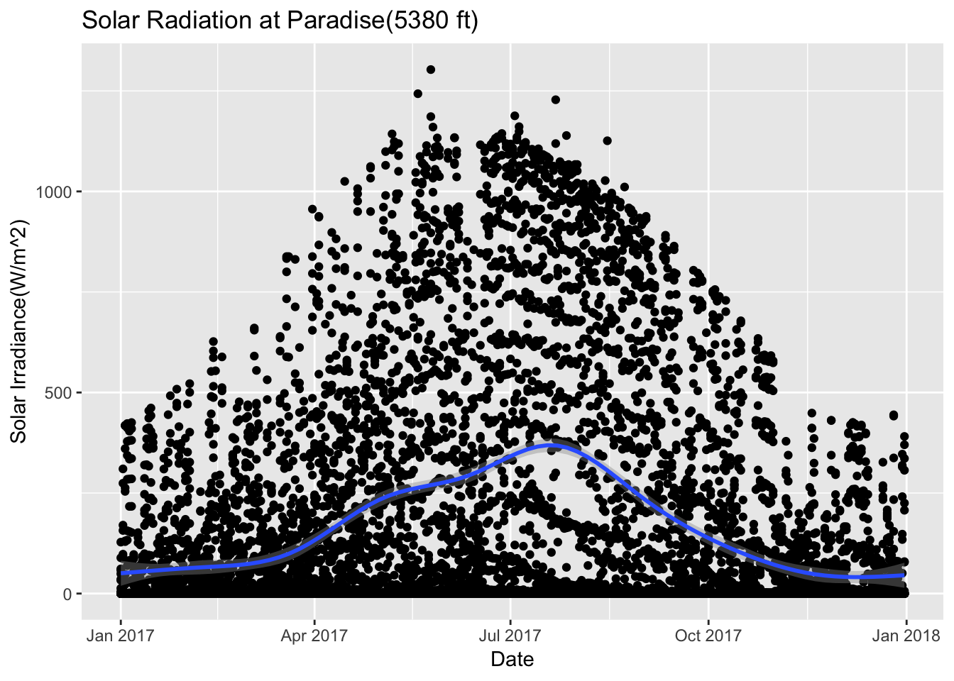
CampMuir_2017 %>% ggplot(aes(date,Solar.Pyranometer..W.m2.)) + geom_point() + stat_smooth(se = TRUE) + ggtitle("Solar Radiation at CampMuir(10110 ft)")+ xlab("Date") + ylab("Solar Irradiance(W/m^2)")## `geom_smooth()` using method = 'gam' and formula 'y ~ s(x, bs = "cs")'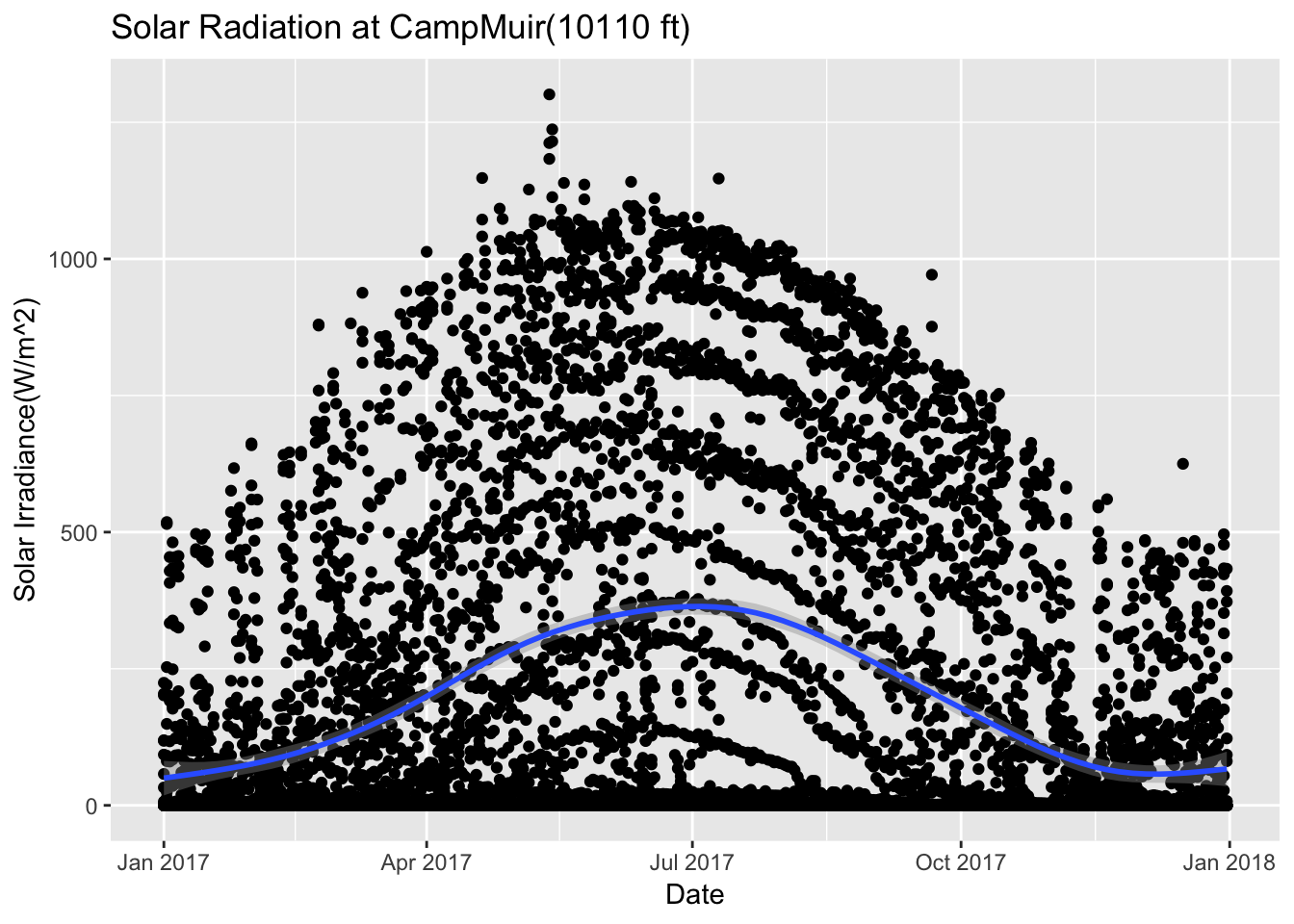
Sunriseupper_2017 %>% ggplot(aes(date,Solar.Pyranometer..W.m2.)) + geom_point() + stat_smooth(se = TRUE) + ggtitle("Solar Radiation at Sunrise-Upper(6880 ft)")+ xlab("Date") + ylab("Solar Irradiance(W/m^2)")## `geom_smooth()` using method = 'gam' and formula 'y ~ s(x, bs = "cs")'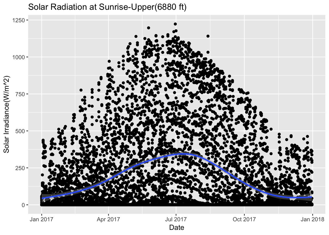
Feedback
Better to do it houry so that daily patterns do confound it. So, now we have hourly solar radiation across all the sites.
## 4-28-2008

#

ggplot(Paradise_2017, aes(hr,Solar.Pyranometer..W.m2.))+
  stat_boxplot( aes(hr,Solar.Pyranometer..W.m2.),
    geom='errorbar', linetype=1, width=0.5)+  #whiskers
  geom_boxplot( aes(hr,Solar.Pyranometer..W.m2.),outlier.shape=1) +
  stat_summary(fun.y=mean, geom="point", size=2) +
  stat_summary(fun.data = mean_se, geom = "errorbar")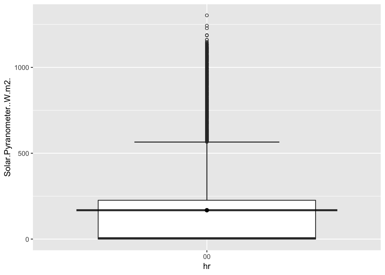
 annotate("text",x=20,y=55,label="wassup!" , family="xkcd"
           )
## mapping: x = ~x, y = ~y
## geom_text: na.rm = FALSE
## stat_identity: na.rm = FALSE
## position_identity## 4-28-2008
#
ggplot(CampMuir_2017, aes(hr,Solar.Pyranometer..W.m2.))+
stat_boxplot( aes(hr,Solar.Pyranometer..W.m2.),
geom='errorbar', linetype=1, width=0.5)+ #whiskers
geom_boxplot( aes(hr,Solar.Pyranometer..W.m2.),outlier.shape=1) +
stat_summary(fun.y=mean, geom="point", size=2) +
stat_summary(fun.data = mean_se, geom = "errorbar")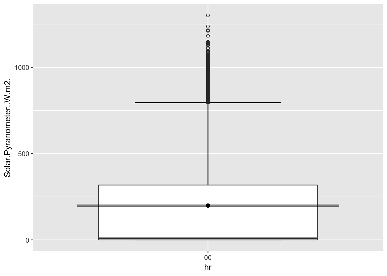
It does confirm that higher the sites, the solar radiation is slightly higher.
8.5 4-29-2008
Lets assume that solar radiation is infact more relevant at higher elevations, so snowmelt would be at a faster rate at higher elevations. Is snowmelt even at all the elevations ? Intuitively no as we often see that peaks hold-on to snow longer. (Just aside discussion).
Here, the goal is to see if there is a difference in radiation recieved at the sites. Reasoning being if the solar radiation recorded is different, that would mean differemt growing degree days. Lets look for June, July and August(JJA Summer). Summer solstice - June 21st.
## 4-29-2008
library(gridExtra)
##
## Attaching package: 'gridExtra'## The following object is masked from 'package:dplyr':
##
## combine#
g1 <- Paradise_2017 %>% filter(month %in% c('06','07','08')) %>% ggplot( aes(hr,Solar.Pyranometer..W.m2.)) + geom_boxplot() +
stat_summary(colour = "red",size=0.5) + theme_classic() +theme(axis.text.x = element_text(angle = 90, hjust = 1)) + xlab("Hour") + ggtitle("Paradise(5k ft) ")
g2 <- CampMuir_2017 %>% filter(month %in% c('06','07','08')) %>% ggplot( aes(hr,Solar.Pyranometer..W.m2.)) + geom_boxplot() +
stat_summary(colour = "red",size=0.5) + theme_classic() +theme(axis.text.x = element_text(angle = 90, hjust = 1)) + xlab("Hour") + ggtitle("Camp Muir(10k ft) ")
grid.arrange(g1, g2,ncol=2, top = "JJA - Mean Hourly Solar Radiation at 2 elevations")## No summary function supplied, defaulting to `mean_se()## No summary function supplied, defaulting to `mean_se()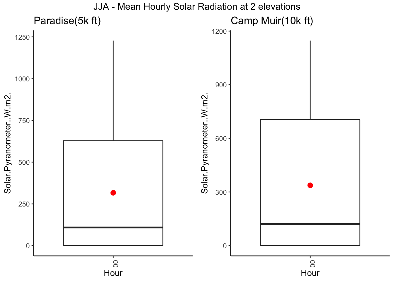
## 4-29-2008
library(gridExtra)
#


g3 <- Paradise_2017 %>%  filter(month %in% c('06')) %>% ggplot( aes(hr,Solar.Pyranometer..W.m2.)) + geom_boxplot() +
    theme_classic() +theme(axis.text.x = element_text(angle = 90, hjust = 1)) +     xlab("Hour") + ggtitle("Paradise(5k ft) ")


g4 <- CampMuir_2017 %>%  filter(month %in% c('06')) %>% ggplot( aes(hr,Solar.Pyranometer..W.m2.)) + geom_boxplot() +
   theme_classic() +theme(axis.text.x = element_text(angle = 90, hjust = 1)) +     xlab("Hour") + ggtitle("Camp Muir(10k ft) ")


grid.arrange(g3, g4,ncol=2, top = "June - Max Hourly Solar Radiation at 2 elevations")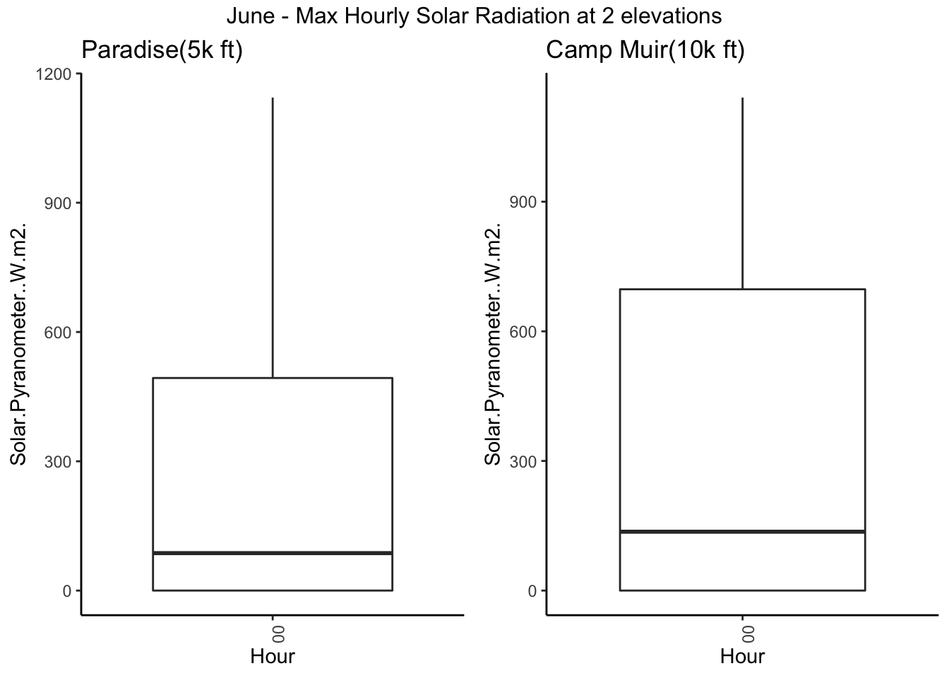
#ggplotly()Lets check the daily max for each day in summer(JJA)
## 4-29-2008
library(gridExtra)
#


g5 <- Paradise_2017 %>%  filter(month %in% c('06','07','08')) %>% dplyr::group_by(date) %>%
  dplyr::summarise(maxSol = max(Solar.Pyranometer..W.m2.)) %>%
  ggplot( aes(date,maxSol)) + geom_point() + geom_line() +
    theme_classic() +theme(axis.text.x = element_text(angle = 90, hjust = 1)) +     xlab("Date") + ggtitle("Paradise(5k ft) ")


g6 <- CampMuir_2017 %>%  filter(month %in% c('06','07','08')) %>% dplyr::group_by(date) %>%
  dplyr::summarise(maxSol = max(Solar.Pyranometer..W.m2.)) %>%
  ggplot( aes(date,maxSol)) + geom_point() +  geom_line() +
    theme_classic() +theme(axis.text.x = element_text(angle = 90, hjust = 1)) +     xlab("Date") + ggtitle("Camp Muir(10k ft) ")


grid.arrange(g5, g6,ncol=2, top = "JJA - Daily Max Solar Radiation at 2 elevations")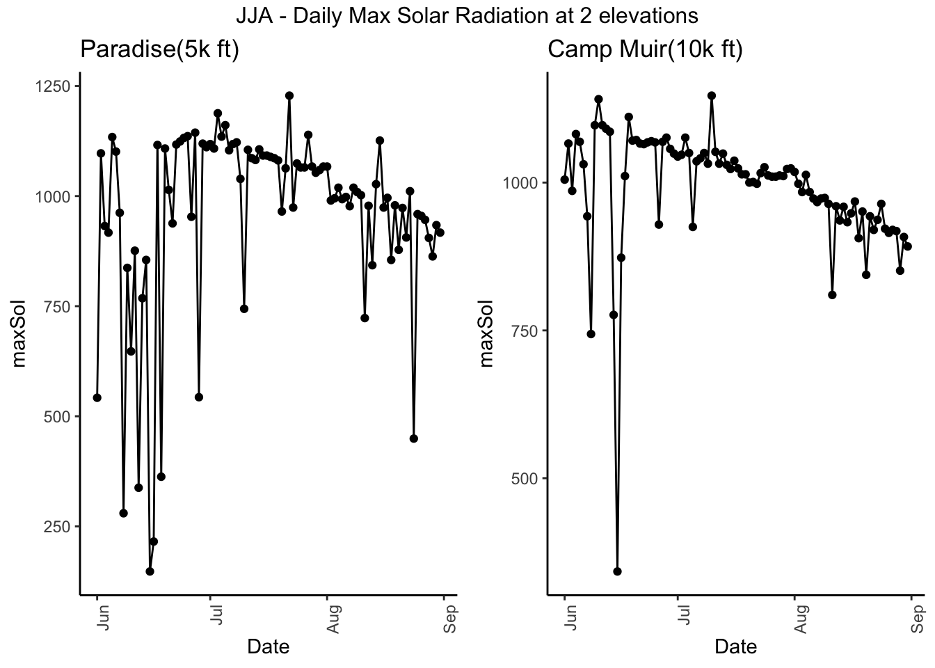
#ggplotly()Compare wind and solar at two sites
## 4-29-2008
library(gridExtra)
#


g5 <- Paradise_2017 %>%  filter(month %in% c('06','07','08')) %>% dplyr::group_by(date) %>%
  dplyr::summarise(maxSol = max(Solar.Pyranometer..W.m2.),maxWind = max(Wind.Speed.Average..mph.)) %>%
  ggplot() + geom_line(aes(date,log(maxSol),color='log Solar(W/m^2)') ) + geom_line(aes(date,maxWind,color='Wind(m/h)')) +
    theme_classic() +theme(axis.text.x = element_text(angle = 90, hjust = 1)) +     xlab("Date") + ylab("") + ggtitle("Paradise(5k ft) ") + scale_color_discrete(name="Variable")


g6 <- CampMuir_2017 %>%  filter(month %in% c('06','07','08')) %>% dplyr::group_by(date) %>%
  dplyr::summarise(maxSol = max(Solar.Pyranometer..W.m2.),maxWind = max(Wind.Speed.Average..mph.)) %>%
  ggplot() + geom_line(aes(date,log(maxSol),color='log Solar(W/m^2)') ) + geom_line(aes(date,maxWind,color='Wind(m/h)')) +
    theme_classic() +theme(axis.text.x = element_text(angle = 90, hjust = 1)) +     xlab("Date") + ylab("") + ggtitle("Camp Muir(10k ft) ") + scale_color_discrete(name="Variable")


grid.arrange(g5, g6,ncol=2, top = "JJA - Daily Max Solar and Max Wind(Avg)  at 2 elevations")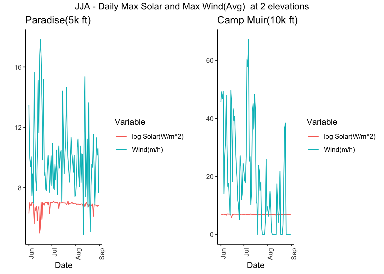
#ggplotly()8.6 5-21-2018
Wrangle the microclimate data
## 5-21-2018
mclim_2018<- read.csv('./data/DATALOG.5.15.2018.csv')

#ggplotly()
Look at the data
## 5-21-2018
str(mclim_2018)
## 'data.frame': 326489 obs. of 4 variables:
## $ X2018.5.8.16.35.01: Factor w/ 73277 levels "2018/5/10 0:00:03",..: 60336 60336 60336 60336 60336 60337 60338 60338 60338 60338 ...
## $ X28CF6F0400008059 : Factor w/ 6 levels "287F5B04000080C5",..: 1 5 6 4 3 2 1 5 6 4 ...
## $ X14.31 : num 14.8 14.4 14.8 14.3 14.1 ...
## $ X4.14 : num 4.14 4.14 4.14 4.14 4.14 4.14 4.14 4.14 4.14 4.14 ...names(mclim_2018) <- c('time','nodeid','temp','batt')
mclim_2018$time <- as.POSIXct(mclim_2018$time, "%Y/%m/%d %H:%M:%S")Add Hour, month and day
## 5-21-2018
mclim_2018$hr <- hour(mclim_2018$time)
mclim_2018$day <- day(mclim_2018$time)
mclim_2018$month<- month(mclim_2018$time)
Basic plot (May 10th)
## 5-21-2018
mclim_2018 %>% filter(day(time) %in% '10') %>%
ggplot( aes(time,temp,color = nodeid)) + geom_line() + theme_minimal()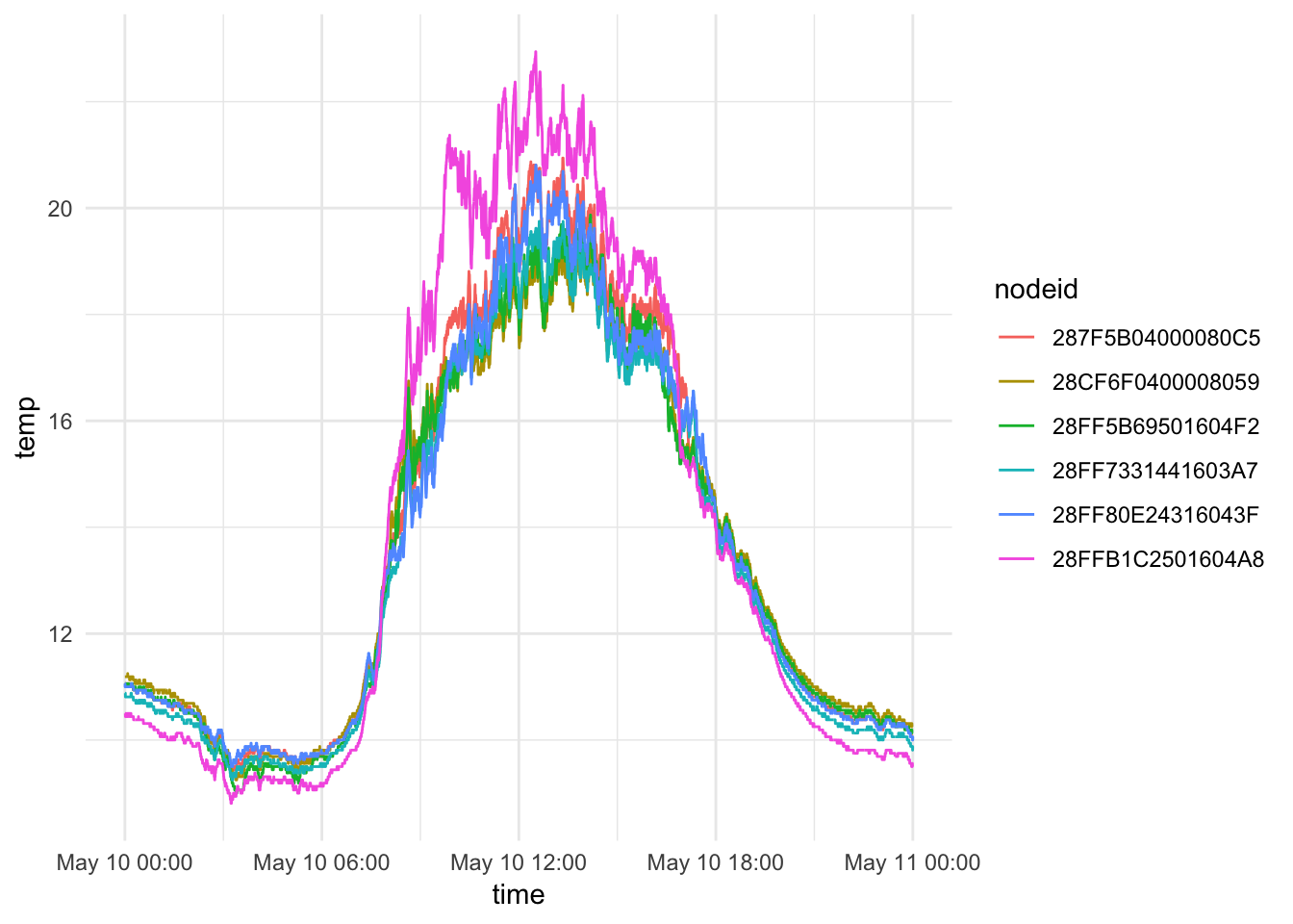
#ggplotly()Whole week
## 5-21-2018
mclim_2018 %>%
ggplot( aes(time,temp,color = nodeid)) + geom_line()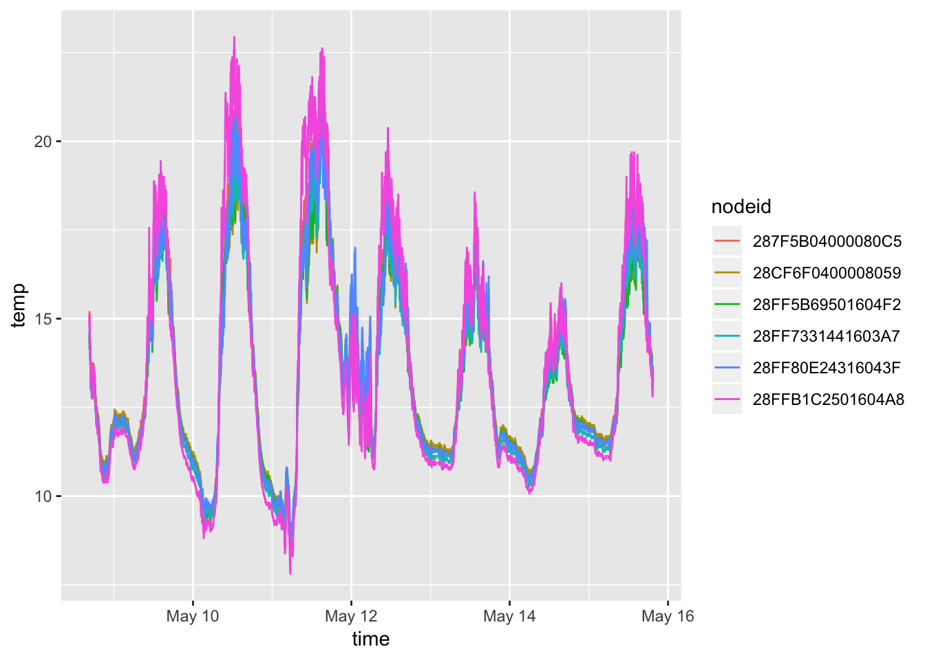
#ggplotly()Add heights (Roghly .25 m apart)
mclim_2018$height <- 0

mclim_2018[mclim_2018$nodeid=='28FF80E24316043F' ,]$height <- 0.25
mclim_2018[mclim_2018$nodeid=='28FF7331441603A7' ,]$height <- 0.5
mclim_2018[mclim_2018$nodeid=='287F5B04000080C5' ,]$height <- 0.75
mclim_2018[mclim_2018$nodeid=='28FFB1C2501604A8' ,]$height <- 1
mclim_2018[mclim_2018$nodeid=='28CF6F0400008059' ,]$height <-1.25
mclim_2018[mclim_2018$nodeid=='28FF5B69501604F2' ,]$height <- 1.5
Basic plot (May 10th) - By height
## 5-21-2018
mclim_2018 %>% filter(day(time) %in% '10') %>%
ggplot( aes(time,temp,color = factor(height))) + geom_line() + theme_minimal()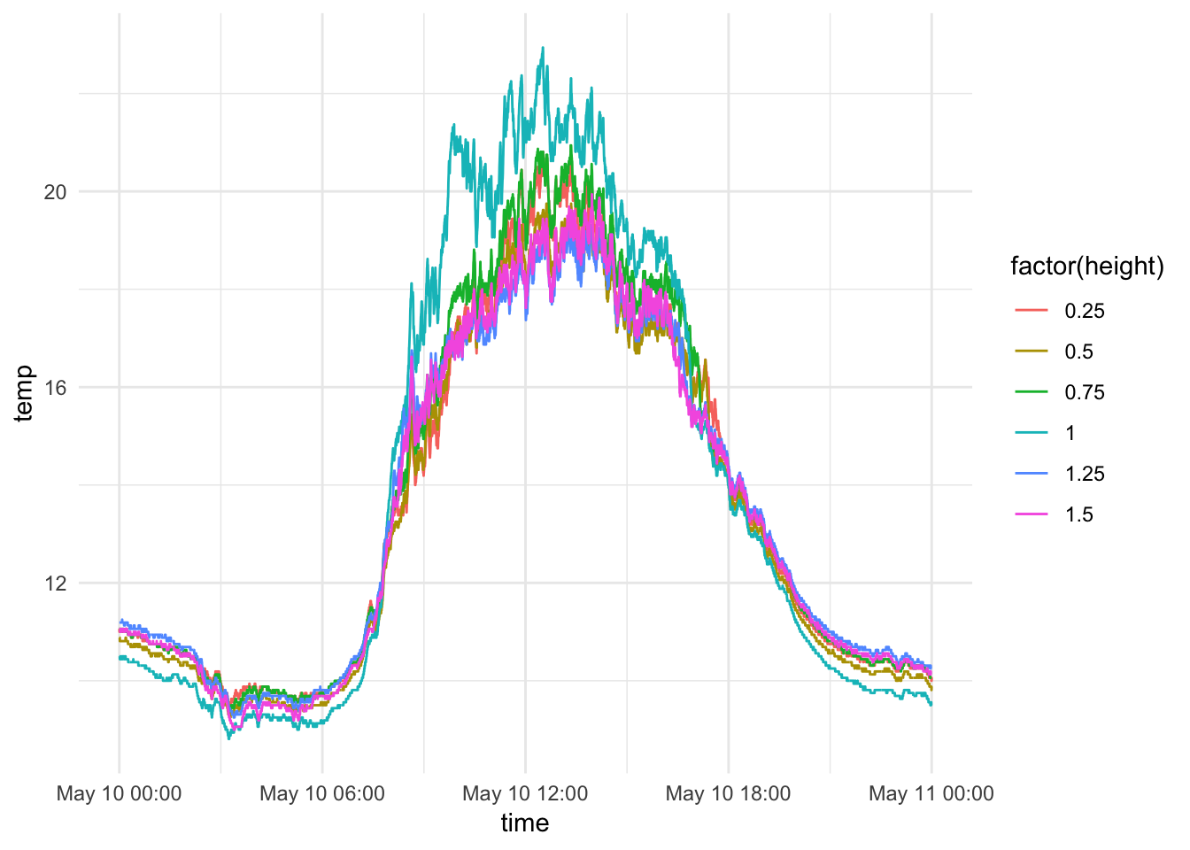
#ggplotly()Add simulated wind profile
mclim_2018$ws <- 0
mclim_2018[mclim_2018$nodeid=='287F5B04000080C5',]$ws <- 4.34
mclim_2018[mclim_2018$nodeid=='28FF80E24316043F' ,]$ws <- 2.02
mclim_2018[mclim_2018$nodeid=='28FFB1C2501604A8' ,]$ws <- 5.20
mclim_2018[mclim_2018$nodeid=='28FF7331441603A7' ,]$ws <- 3.45
mclim_2018[mclim_2018$nodeid=='28FF5B69501604F2' ,]$ws <- 7.56
mclim_2018[mclim_2018$nodeid=='28CF6F0400008059' ,]$ws <-6.54
Redo the plot by height
## 5-21-2018
mclim_2018 %>% filter(day(time) %in% '10', height %in% c(0.25,1)) %>%
ggplot( aes(time,temp,color = factor(height))) + geom_line() + theme_minimal()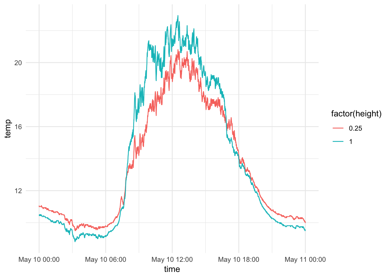
Redo the plot by height for Wind Speed
## 5-21-2018
mclim_2018 %>% filter(day(time) %in% '10', height %in% c(0.25,0.5,0.75,1)) %>%
ggplot( aes(time,ws,color = factor(height))) + geom_line() + theme_minimal()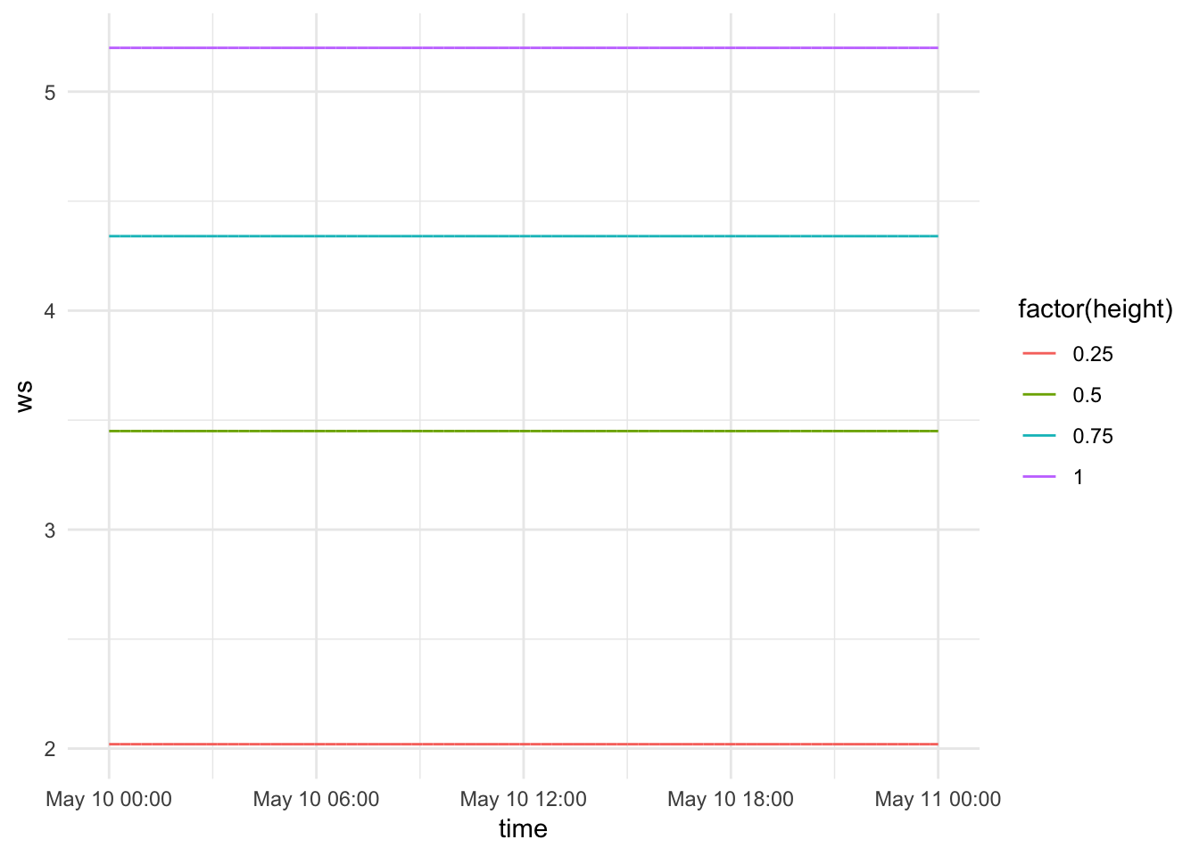
Calculate (Wind speed at any height = U_star/K*log(Z/Z0))
Calculate zero plane displcement
#TODO - Do by each hour
zeroDM<- lm(log(mclim_2018$height) ~ mclim_2018$ws)
zD <- exp(zeroDM$coeff[1])
#.16
Calculate roughness and Z*
#With zero plane dispacement
sRM<- lm(mclim_2018$ws ~ log(mclim_2018$height-zD))

srIntercept <- sRM$coeff[1]
srSlope <- sRM$coeff[2]

K=0.4 # Von Karman constant

z0<-  exp(-srIntercept/srSlope) #0.04
U_star<-  srSlope*K
Repeat this for each site ## 7-21-2018
#With zero plane dispacement
library(rgdal) #this package is necessary to import the .asc file in R.
## rgdal: version: 1.4-4, (SVN revision 833)
## Geospatial Data Abstraction Library extensions to R successfully loaded
## Loaded GDAL runtime: GDAL 2.1.3, released 2017/20/01
## Path to GDAL shared files: /Library/Frameworks/R.framework/Versions/3.6/Resources/library/rgdal/gdal
## GDAL binary built with GEOS: FALSE
## Loaded PROJ.4 runtime: Rel. 4.9.3, 15 August 2016, [PJ_VERSION: 493]
## Path to PROJ.4 shared files: /Library/Frameworks/R.framework/Versions/3.6/Resources/library/rgdal/proj
## Linking to sp version: 1.3-1library(rasterVis) #this package has the function which allows the 3D plotting.## Loading required package: raster##
## Attaching package: 'raster'## The following object is masked from 'package:ggpubr':
##
## rotate## The following object is masked from 'package:magrittr':
##
## extract## The following object is masked from 'package:plotly':
##
## select## The following object is masked from 'package:dplyr':
##
## select## The following object is masked from 'package:tidyr':
##
## extract## Loading required package: lattice## Loading required package: latticeExtra## Loading required package: RColorBrewer##
## Attaching package: 'latticeExtra'## The following object is masked from 'package:ggplot2':
##
## layer#set the path where the file is, and import it into R.
r= raster(paste("./data/rainier_2012_dtm_5_hs.tif", sep=""))
#visualize the raster in 3D
plot(r,lit=TRUE)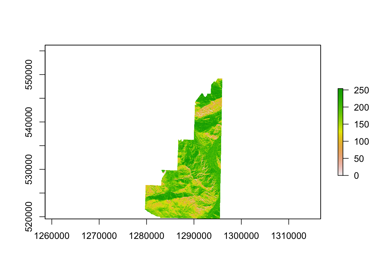 Combining multiple rasters into one single file.
fs <- list.files(path="./data", pattern = "rainier_2007_*", full.names = TRUE)
library(raster)

r1 <- raster(fs[1])
r2 <- raster(fs[2])
r3 <- raster(fs[3])
r4 <- raster(fs[4])
r5 <- raster(fs[5])
r6 <- raster(fs[6])
r7 <- raster(fs[7])
r8 <- raster(fs[8])
r9 <- raster(fs[9])
r10 <- raster(fs[10])
r11 <- raster(fs[11])
r12 <- raster(fs[12])
r13 <- raster(fs[13])
r14 <- raster(fs[14])
r15 <- raster(fs[15])
r16 <- raster(fs[16])
r17 <- raster(fs[17])

# if you have a list of Raster objects, you can use do.call
x <- list(r1, r2, r3,r4,r5,r6,r7,r8,r9,r10,r11,r12,r13,r14,r15,r16,r17)
names(x)[1:2] <- c('x', 'y')
x$fun <- mean
x$na.rm <- TRUE

#y <- do.call(mosaic, x)

#writeRaster(y, "./data/combined_mtr.TIF")
##7-25-2018
Check the diurnal variation for summer, using Paradise as a proxy
Paradise_2017 %>% group_by(date,month,hr) %>% ggplot(aes(month,Solar.Pyranometer..W.m2.)) + geom_point() 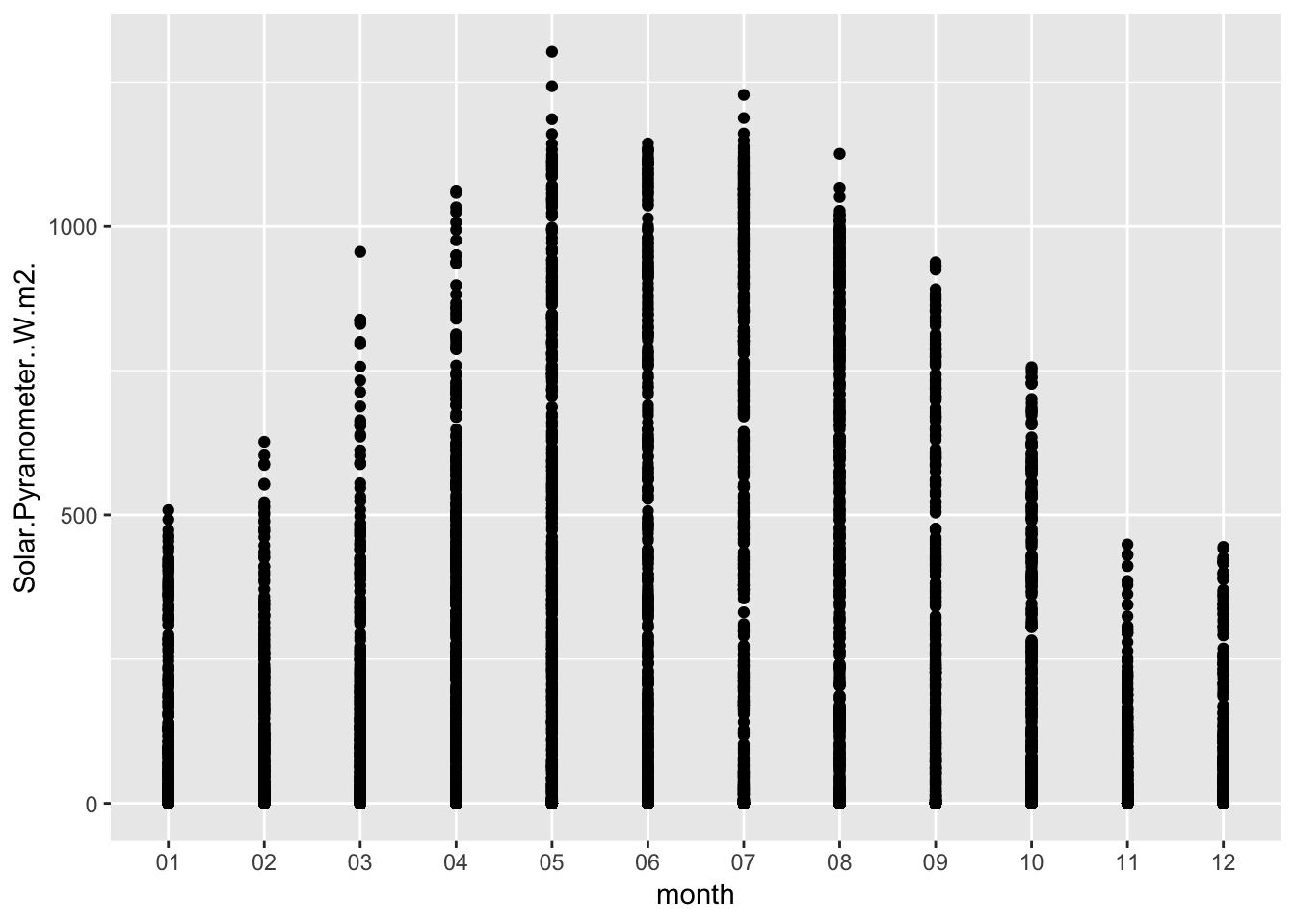
#.16Use SNOTEL data from Paradise(Latitude: 46.78 Longitude: -121.74)
Check the diurnal variation for summer, using Paradise as a proxy
Paradise_Snotel_2013<- read.csv('./data/679_STAND_WATERYEAR=2013.csv')
Paradise_Snotel_2013$date <- as.Date(Paradise_Snotel_2013$Date, "%Y-%m-%d")
Paradise_Snotel_2013$month <- strftime(Paradise_Snotel_2013$Date,'%m')

Paradise_Snotel_2012<- read.csv('./data/679_STAND_WATERYEAR=2012.csv')
Paradise_Snotel_2012$date <- as.Date(Paradise_Snotel_2012$Date, "%Y-%m-%d")
Paradise_Snotel_2012$month <- strftime(Paradise_Snotel_2012$Date,'%m')

Paradise_Snotel_2011<- read.csv('./data/679_STAND_WATERYEAR=2011.csv')
Paradise_Snotel_2011$date <- as.Date(Paradise_Snotel_2011$Date, "%Y-%m-%d")
Paradise_Snotel_2011$month <- strftime(Paradise_Snotel_2011$Date,'%m')

Paradise_Snotel_2013 %>% group_by(date,month) %>% mutate(diva=TMAX.D.1..degC.-TMIN.D.1..degC.)%>% ggplot() + geom_line(aes(date,TMIN.D.1..degC.,colour='min'))  +geom_line(aes(date,TMAX.D.1..degC.,colour='max')) +geom_line(aes(date,diva,colour='diurnal variation'))+ theme_minimal()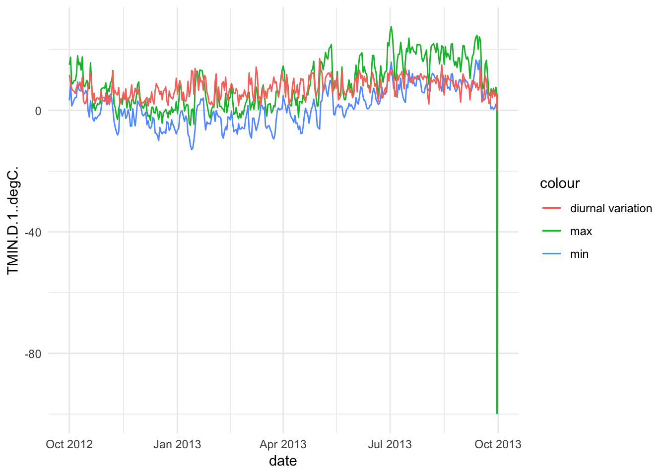
#.16Only Summer
Paradise_Snotel_2013 %>% group_by(date,month) %>% filter(as.numeric(month) %in% c(6,7,8)) %>% mutate(diva=TMAX.D.1..degC.-TMIN.D.1..degC.)%>% ggplot() + geom_line(aes(date,TMIN.D.1..degC.,colour='min')) +geom_line(aes(date,TMAX.D.1..degC.,colour='max'))+geom_line(aes(date,TAVG.D.1..degC.,colour='avg')) +geom_line(aes(date,diva,colour='diurnal variation'))+ theme_minimal() +xlab("Date") + ylab("") + ggtitle("Snotel Paradise - Water year 2013 ") + scale_color_discrete(name="Metric")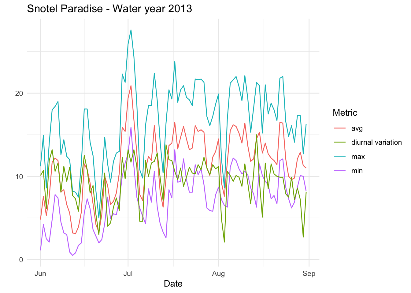
#.16For 2012
Paradise_Snotel_2012 %>% group_by(date,month) %>% filter(as.numeric(month) %in% c(6,7,8) & TMIN.D.1..degC. != -99.9) %>% mutate(diva=TMAX.D.1..degC.-TMIN.D.1..degC.)%>% ggplot() + geom_line(aes(date,TMIN.D.1..degC.,colour='min')) +geom_line(aes(date,TMAX.D.1..degC.,colour='max'))+geom_line(aes(date,TAVG.D.1..degC.,colour='avg')) +geom_line(aes(date,diva,colour='diurnal variation'))+ theme_minimal() +xlab("Date") + ylab("") + ggtitle("Snotel Paradise - Water year 2012 ") + scale_color_discrete(name="Metric")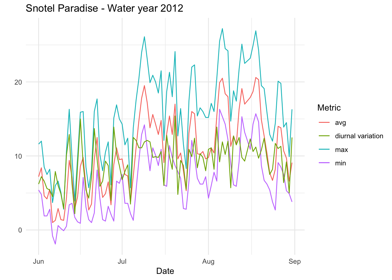
#.16For 2011
Paradise_Snotel_2011 %>% group_by(date,month) %>% filter(as.numeric(month) %in% c(6,7,8)) %>% mutate(diva=TMAX.D.1..degC.-TMIN.D.1..degC.)%>% ggplot() + geom_line(aes(date,TMIN.D.1..degC.,colour='min')) +geom_line(aes(date,TMAX.D.1..degC.,colour='max'))+geom_line(aes(date,TAVG.D.1..degC.,colour='avg')) +geom_line(aes(date,diva,colour='diurnal variation'))+ theme_minimal() +xlab("Date") + ylab("") + ggtitle("Snotel Paradise - Water year 2011 ") + scale_color_discrete(name="Metric")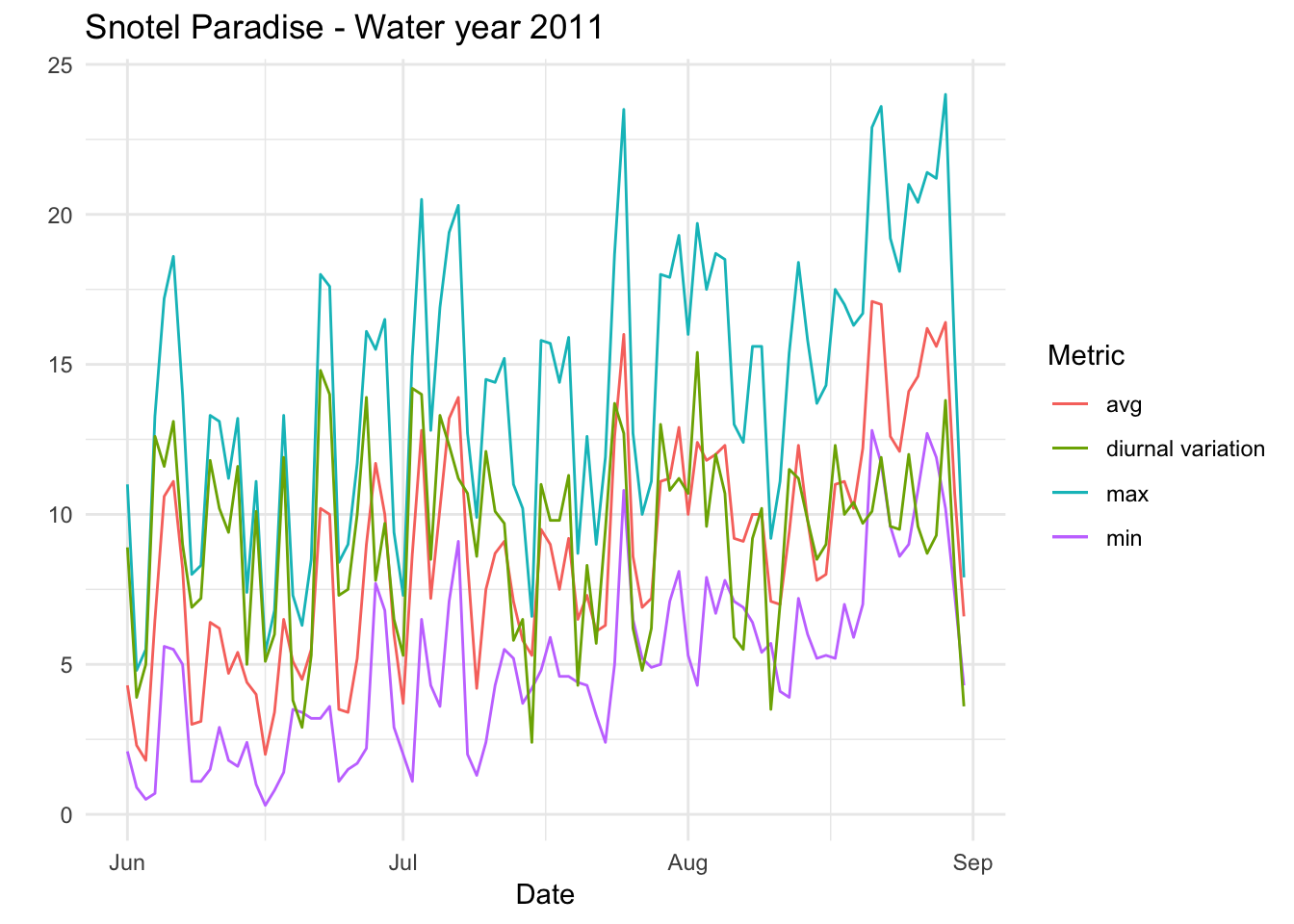
#.168.7 7-26-2018
Lets look at the diurnal variation for three months, need to switch to NWAC as Snotel does not provide hourly breakdown
Paradise_5400_2017<- read.csv('./data/Paradise_5400_feet_2017.csv')
Paradise_5400_2016<- read.csv('./data/Paradise_5400_feet_2016.csv')
Paradise_5400_2015<- read.csv('./data/Paradise_5400_feet_2015.csv')

Paradise_5400_2017$date <- as.Date(Paradise_5400_2017$Date.Time..PST., "%Y-%m-%d")
Paradise_5400_2017$datetime <- as.Date(Paradise_5400_2017$Date.Time..PST., "%Y-%m-%d %H:%M")
library(lubridate)
library(gridExtra)
Paradise_5400_2017$hr <-lubridate::hour(lubridate::as_datetime(Paradise_5400_2017$Date.Time..PST.))
Paradise_5400_2017$year <-lubridate::year(lubridate::as_datetime(Paradise_5400_2017$Date.Time..PST.))
Paradise_5400_2017$mnth <-lubridate::month(lubridate::as_datetime(Paradise_5400_2017$Date.Time..PST.))
Paradise_5400_2017$min <-lubridate::minute(lubridate::as_datetime(Paradise_5400_2017$Date.Time..PST.))
Paradise_5400_2017$month <- strftime(Paradise_5400_2017$Date.Time..PST.,'%m')
Paradise_5400_2017$day <-strftime(Paradise_5400_2017$Date.Time..PST.,'%d')

Paradise9<- Paradise_5400_2017 %>% group_by(date,month,day,hr) %>% filter(as.numeric(month) %in% c(7,8,9) & as.numeric(day) %in% c(9) ) %>%  ggplot() +  geom_line(aes(as.numeric(hr),Temperature..deg.F.,group=month,color=month)) + theme_minimal() +xlab("Hour") + ylab("Temperature") + ggtitle("Paradise 5400 NWAC - Calendar year 2017  - 9th day") + scale_color_discrete(name="Month")
Paradise16<- Paradise_5400_2017 %>% group_by(date,month,day,hr) %>% filter(as.numeric(month) %in% c(7,8,9) & as.numeric(day) %in% c(16) ) %>%  ggplot() +  geom_line(aes(as.numeric(hr),Temperature..deg.F.,group=month,color=month)) + theme_minimal() +xlab("Hour") + ylab("Temperature") + ggtitle("Paradise 5400 NWAC - Calendar year 2017  - 16th day") + scale_color_discrete(name="Month")
Paradise23<- Paradise_5400_2017 %>% group_by(date,month,day,hr) %>% filter(as.numeric(month) %in% c(7,8,9) & as.numeric(day) %in% c(23) ) %>%  ggplot() +  geom_line(aes(as.numeric(hr),Temperature..deg.F.,group=month,color=month)) + theme_minimal() +xlab("Hour") + ylab("Temperature") + ggtitle("Paradise 5400 NWAC - Calendar year 2017  - 23rd day") + scale_color_discrete(name="Month")

grid.arrange(Paradise9,Paradise16,Paradise23)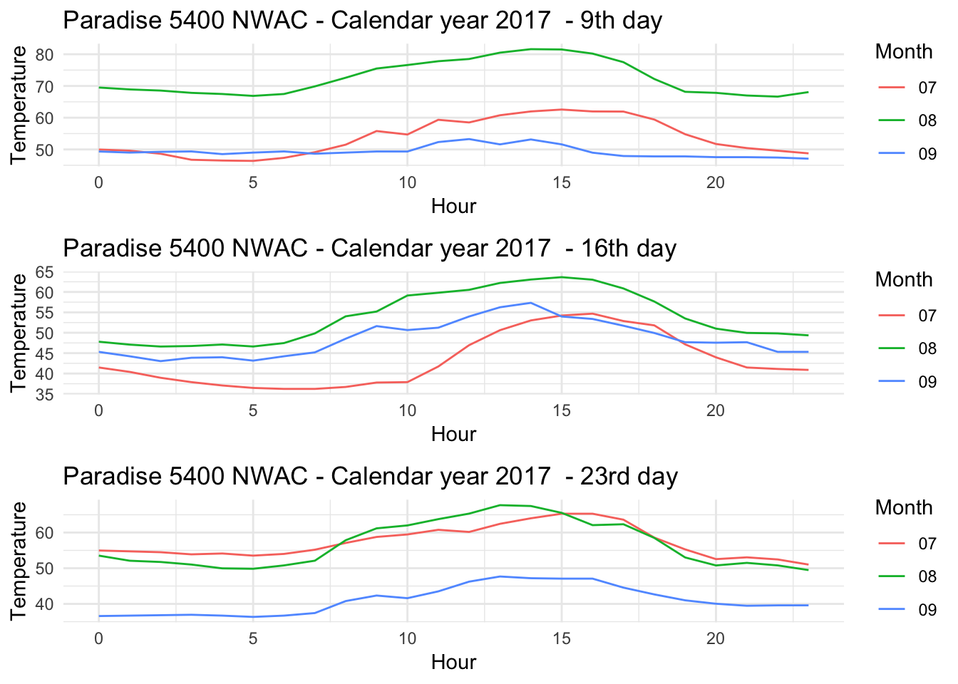
Days overlapping eath other
Paradise_5400_2017 %>% group_by(date,month,day,hr) %>% filter(as.numeric(month) %in% c(7,8,9) & as.numeric(day) %in% c(15,16,17,18,19,20) ) %>% ggplot() + geom_point(aes(as.numeric(hr),Temperature..deg.F.,shape=day,group=7,color=month)) + theme_minimal() +xlab("Hour") + ylab("Temperature") + ggtitle("Paradise 5400 NWAC - Calendar year 2017 - Days(15-20) ") + scale_color_discrete(name="Month")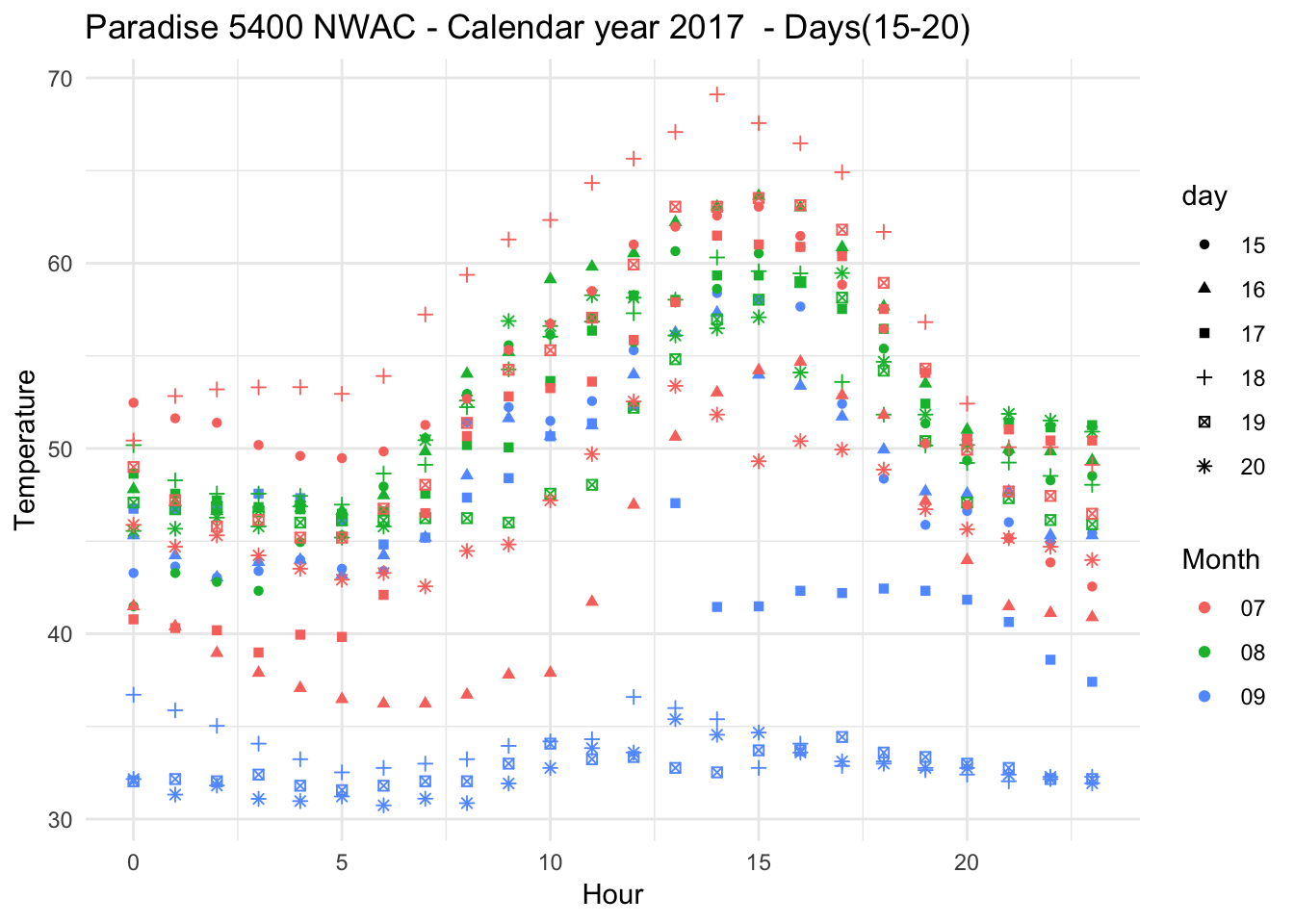
Removing symbols, each line representing different day of the month
Paradise_5400_2017 %>% group_by(date,month,day,hr) %>% filter(as.numeric(month) %in% c(7,8,9) & as.numeric(day) %in% c(15,16,17,18,19,20) ) %>% ggplot(aes(x = hr, y = Temperature..deg.F.,color=month)) + geom_line(data = subset(Paradise_5400_2017,month %in% c("07") & day %in% c("15")  ))+ geom_line(data = subset(Paradise_5400_2017,month %in% c("08") & day %in% c("15")  ))+ geom_line(data = subset(Paradise_5400_2017,month %in% c("09") & day %in% c("15")  ))  +
geom_line(data = subset(Paradise_5400_2017,month %in% c("07") & day %in% c("16")  ))+ geom_line(data = subset(Paradise_5400_2017,month %in% c("08") & day %in% c("16")  ))+ geom_line(data = subset(Paradise_5400_2017,month %in% c("09") & day %in% c("16")  ))  +
geom_line(data = subset(Paradise_5400_2017,month %in% c("07") & day %in% c("17")  ))+ geom_line(data = subset(Paradise_5400_2017,month %in% c("08") & day %in% c("17")  ))+ geom_line(data = subset(Paradise_5400_2017,month %in% c("09") & day %in% c("17")  ))  +
geom_line(data = subset(Paradise_5400_2017,month %in% c("07") & day %in% c("18")  ))+ geom_line(data = subset(Paradise_5400_2017,month %in% c("08") & day %in% c("18")  ))+ geom_line(data = subset(Paradise_5400_2017,month %in% c("09") & day %in% c("18")  ))  +
geom_line(data = subset(Paradise_5400_2017,month %in% c("07") & day %in% c("19")  ))+ geom_line(data = subset(Paradise_5400_2017,month %in% c("08") & day %in% c("19")  ))+ geom_line(data = subset(Paradise_5400_2017,month %in% c("09") & day %in% c("19")  ))  +
geom_line(data = subset(Paradise_5400_2017,month %in% c("07") & day %in% c("20")  ))+ geom_line(data = subset(Paradise_5400_2017,month %in% c("08") & day %in% c("20")  ))+ geom_line(data = subset(Paradise_5400_2017,month %in% c("09") & day %in% c("20")  ))  +
theme_minimal() + xlab("Hour") + ylab("Temperature") + ggtitle("Paradise 5400 NWAC - Calendar year 2017  - Days(15-18) ") + scale_color_discrete(name="Month")+geom_jitter()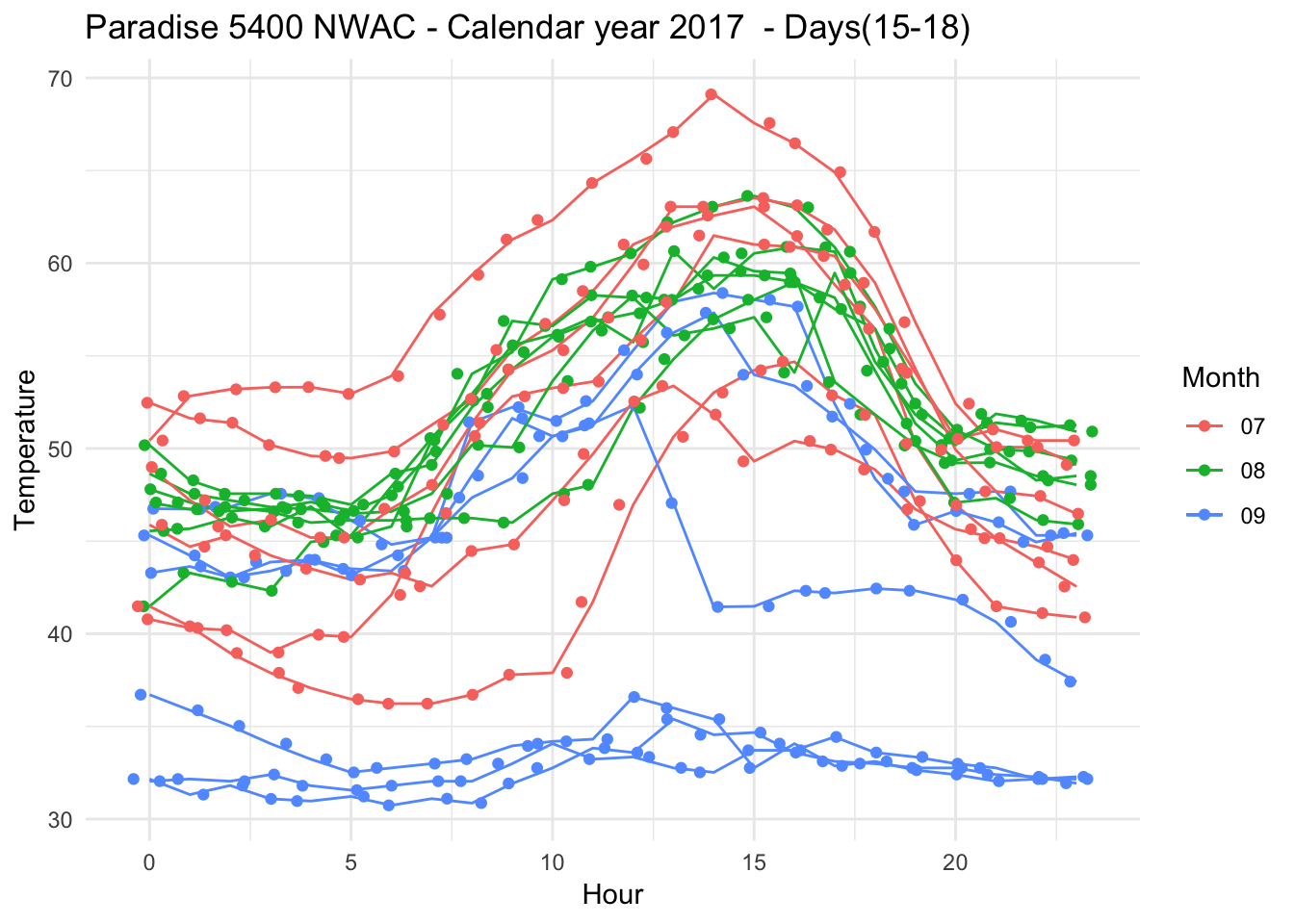
Removing symbols, point plot
Paradise_5400_2017 %>% group_by(date,month,day,hr) %>% filter(as.numeric(month) %in% c(7,8,9) & as.numeric(day) %in% c(15,16,17,18,19,20) ) %>% ggplot(aes(x = hr, y = Temperature..deg.F.,color=month)) + geom_point(data = subset(Paradise_5400_2017,month %in% c("07") & day %in% c("15","16","17","18","19","20")))+ geom_point(data = subset(Paradise_5400_2017,month %in% c("08") & day %in% c("15","16","17","18","19","20") ))+ geom_point(data = subset(Paradise_5400_2017,month %in% c("09") & day %in% c("15","16","17","18","19","20") )) +theme_minimal() +xlab("Hour") + ylab("Temperature") + ggtitle("Paradise 5400 NWAC - Calendar year 2017 - Days(15-18) ") + scale_color_discrete(name="Month")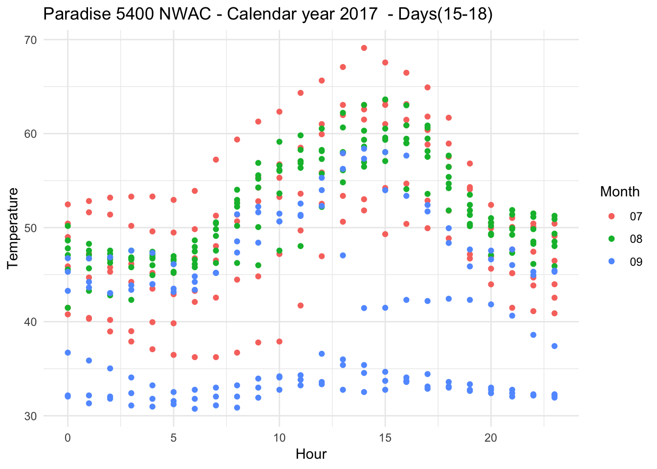
8.8 8-7-2018
One of the arguments in the boundary layer relevance is that at different heights temperature profile varies. So, the vertically the temperature variation differs, and that is bound to influence physiology of organisms living in that strata.
To highlight the point, we could look at microclimate profiled data
Canopy and surface 3 cm vs 103cm
Load the required files
decombined <- read.csv('./data/decombined-1981.csv')library(dplyr)
decombined %>% filter(year(datec) %in% c(1981) & month(datec) %in% c(01) & day(datec) > 12 & day(datec) < 20 ) %>%
dplyr::group_by(month,day,hr) %>% dplyr::summarise(meanST = mean(Tsurface),meanCT = mean(TAH)) %>%
dplyr::group_by(hr) %>% dplyr::summarise(meanST = mean(meanST),meanCT = mean(meanCT)) %>%
ggplot() +
geom_line(aes(hr,meanST-273.5,color='Surface'),se=F)+ geom_line(aes(hr,meanCT-273.5,color='Canopy'),se=F)+
scale_colour_manual("Temperature at", breaks = c("Surface", "Canopy"), values = c("blue","red")) +
theme_minimal() + ggtitle("Variation in temperature at different heights") + xlab("Hour") +
ylab("Temperature(C)") + labs(colour = "Hour",
subtitle="Microclimate impacts at two different heights",caption="Data Source : http://www.microclim.org") 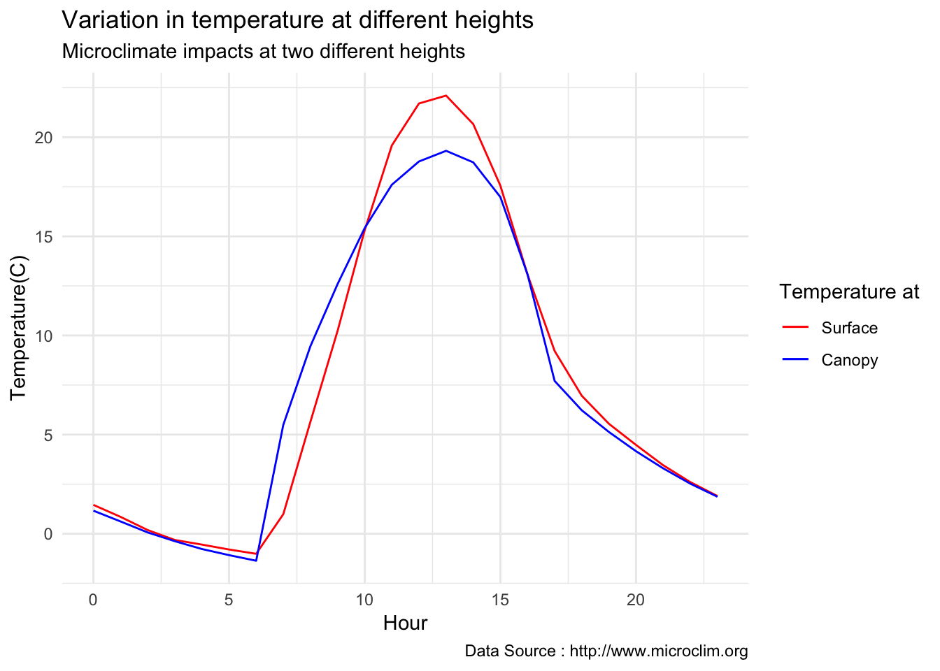
Seasonal temperatures at two heights
library(dplyr)
decombined %>% filter(year(datec) %in% c(1981) & month(datec) %in% c(06,07,08) )  %>%
  dplyr::group_by(month,day,hr) %>% dplyr::summarise(meanST = mean(Tsurface),meanCT = mean(TAH)) %>%
  group_by(hr) %>% dplyr::summarise(meanST = mean(meanST),meanCT = mean(meanCT)) %>%
  ggplot() +
  geom_line(aes(hr,meanST-273.5,color='Surface'),se=F)+ geom_line(aes(hr,meanCT-273.5,color='Canopy'),se=F)+
  scale_colour_manual("Temperature at", breaks = c("Surface", "Canopy"), values = c("blue","red")) +
  theme_minimal() + ggtitle("Seasonal variation in temperature at different heights")  + xlab("Hour") +
  ylab("Temperature (°C)") + labs(colour = "Hour",
subtitle="Microclimate differences at two different heights",caption="Data Source : http://www.microclim.org") 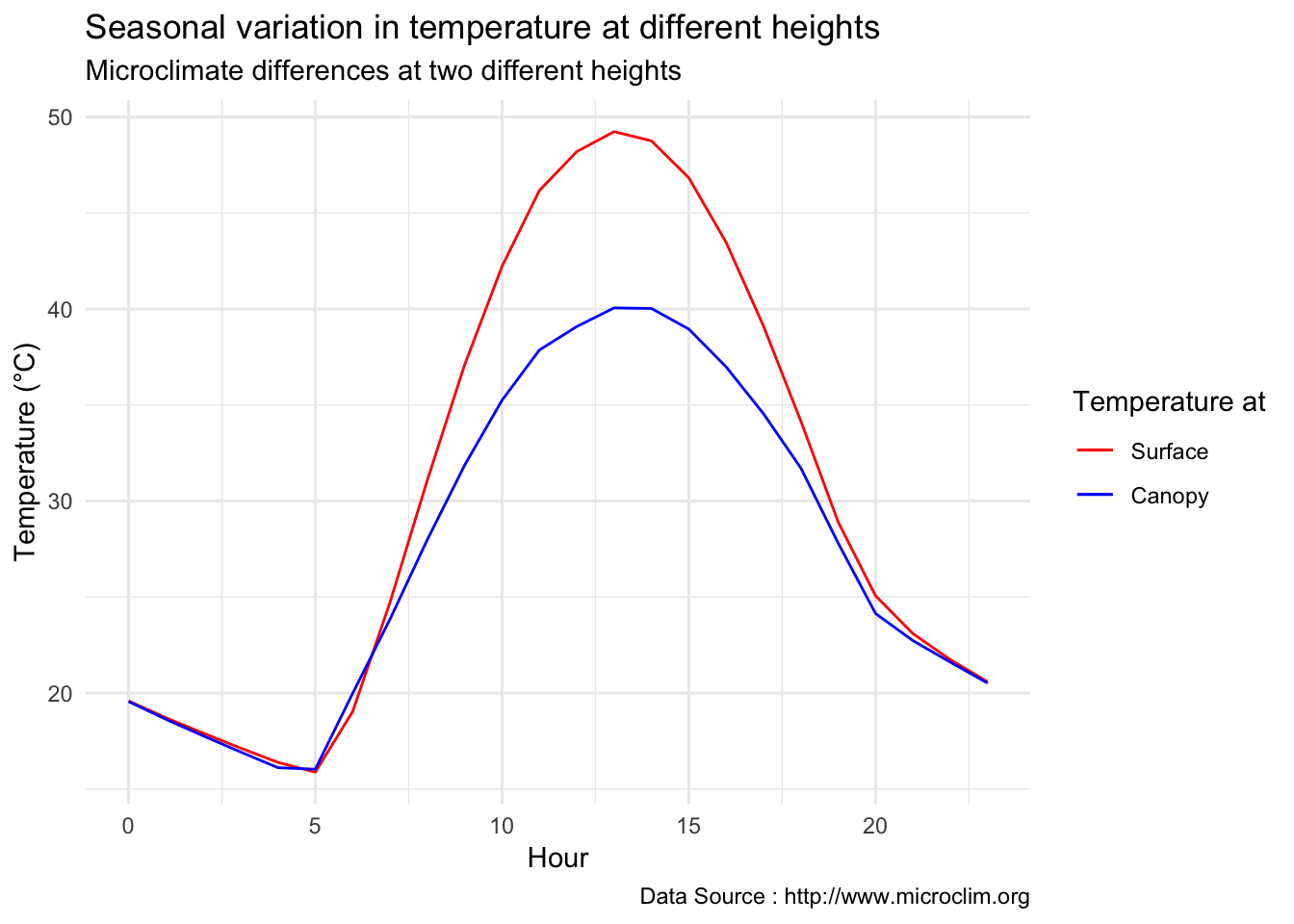
Seasonal difference during peak solar time is phonenomenal, there is almost 10 degree difference.
8.9 8-17-2018
Feedback - Ideal would be to show multiple days plotted on the hourly x-axis to show the variation.
Typical weekly summer variation
decombined %>% filter(year(datec) %in% c(1981) & month(datec) %in% c(01) & day(datec) > 12 & day(datec) < 20 )  %>%
  group_by(month,day,hr)  %>%
  ggplot() +
  geom_line(aes(hr,Tsurface-273.5,group=day,color='Surface'),se=F)+ geom_line(aes(hr,TAH-273.5,group=day ,color='Canopy'),se=F)+
  scale_colour_manual("Temperature at", breaks = c("Surface", "Canopy"), values = c("blue","red")) +
  theme_minimal() + ggtitle("Variation in temperature at two different heights")  + xlab("Hour") +
  ylab("Temperature (°C)") + labs(colour = "Hour",
subtitle="1/13/81 - 1/19/81",caption="Data Source : http://www.microclim.org") 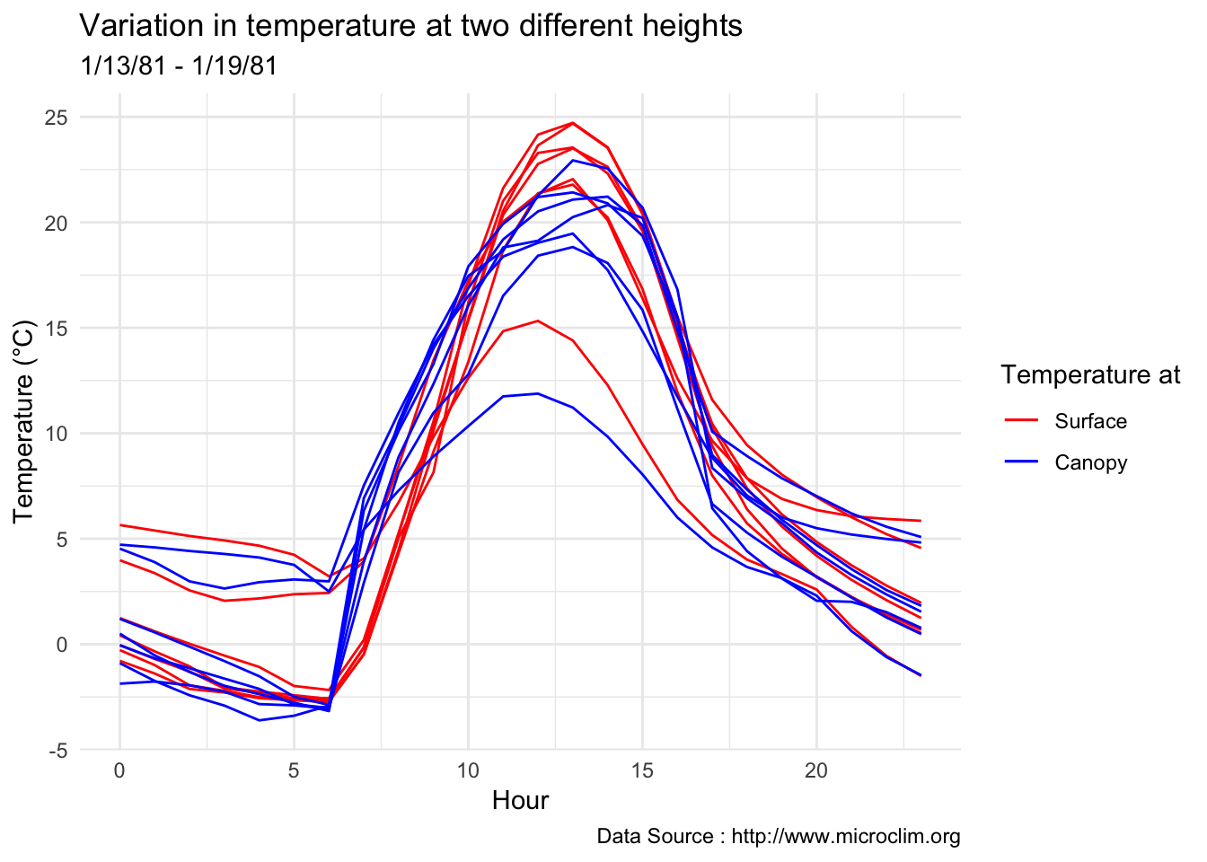
Seasonal temperatures at two heights
decombined %>% filter(year(datec) %in% c(1981) & month(datec) %in% c(06,07,08) )  %>%
  group_by(month,day,hr)  %>%
   ggplot() +
  geom_line(aes(hr,Tsurface-273.5,group=day,color='Surface'),se=F)+ geom_line(aes(hr,TAH-273.5,group=day,color='Canopy'),se=F)+
  scale_colour_manual("Temperature at", breaks = c("Surface", "Canopy"), values = c("blue","red")) +
  theme_minimal() + ggtitle("Seasonal variation in temperature at different heights")  + xlab("Hour") +
  ylab("Temperature (°C)") + labs(colour = "Hour",
subtitle="Microclimate differences at two different heights",caption="Data Source : http://www.microclim.org") 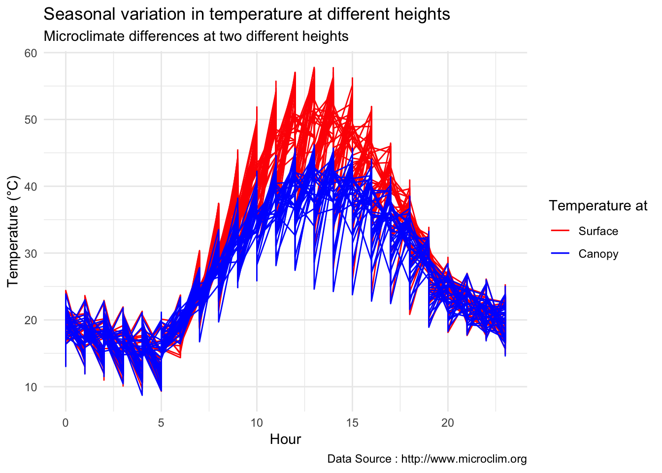
8.10 8-23-2018
Objectives for the day was to have a functional code for CN(Complete Node) and TN(Temperature only node).
KX and AX are here to help me out, just awesome!
We installed one CN with Anemometers, and tested it. The code needed some work, but we were able to bring-up one with four anemometers.
We had three objectives as we were putting the nodes up.
** Have a reliable real-time clock ** Mount the solar radiation sensor on a firm base(there is a bubble to help stablize) ** Have a status indicator to check the activity
8.11 8-24-2018
Few issues overnight.
DS1802B runs on 1-Wire, and on the same bus you can use umpteen number of them. By design, it should have worked, but we had problems with connecting more than four
8.12 9-23-2018
Analysis of data from the first field experiment. Mt Rainier deployment in the forest canopies.
av06_mm <- read_csv('./data/DATALOG-av06-cn.csv')## Parsed with column specification:
## cols(
## date = col_character(),
## temp1 = col_double(),
## temp2 = col_double(),
## temp3 = col_double(),
## temp4 = col_double(),
## windspeed1 = col_double(),
## windspeed2 = col_double(),
## windspeed3 = col_double(),
## windspeed4 = col_double(),
## winddirection1 = col_double(),
## winddirection2 = col_double(),
## winddirection3 = col_double(),
## winddirection4 = col_double(),
## solar = col_double(),
## battery = col_double()
## )str(av06_mm)## Classes 'spec_tbl_df', 'tbl_df', 'tbl' and 'data.frame': 6252 obs. of 15 variables:
## $ date : chr "9/2/18 9:44:7" "9/2/18 9:47:9" "9/2/18 9:50:11" "9/2/18 9:53:12" ...
## $ temp1 : num 20.9 20.9 20.8 20.8 20.7 ...
## $ temp2 : num 21.1 21.1 21.1 21.1 20.9 ...
## $ temp3 : num 21.5 21.4 21.1 21.2 21.2 ...
## $ temp4 : num 20.8 20.8 20.8 20.8 20.8 ...
## $ windspeed1 : num 0 0 0 0 0 0 0 0 0 0 ...
## $ windspeed2 : num 0 0 0 0 0 0 0 0 0 0 ...
## $ windspeed3 : num 0 0 0 0 0 0 0 0 0 0 ...
## $ windspeed4 : num 0 0 0 0 0 0 0 0 0 0 ...
## $ winddirection1: num 1007 1009 1006 1010 1012 ...
## $ winddirection2: num 953 953 955 953 957 958 953 959 957 959 ...
## $ winddirection3: num 1004 1007 1004 1007 1008 ...
## $ winddirection4: num 979 975 976 974 977 976 979 974 973 973 ...
## $ solar : num 1022 1022 1021 1022 1023 ...
## $ battery : num 4.18 4.18 4.18 4.18 4.18 4.18 4.18 4.18 4.18 4.18 ...
## - attr(*, "spec")=
## .. cols(
## .. date = col_character(),
## .. temp1 = col_double(),
## .. temp2 = col_double(),
## .. temp3 = col_double(),
## .. temp4 = col_double(),
## .. windspeed1 = col_double(),
## .. windspeed2 = col_double(),
## .. windspeed3 = col_double(),
## .. windspeed4 = col_double(),
## .. winddirection1 = col_double(),
## .. winddirection2 = col_double(),
## .. winddirection3 = col_double(),
## .. winddirection4 = col_double(),
## .. solar = col_double(),
## .. battery = col_double()
## .. )Plot four temperatures
tp <- av06_mm %>% dplyr::mutate(row_no= row_number()) %>% ggplot() +
  geom_line(aes(row_no,temp1,color='red')) +
  geom_line(aes(row_no,temp2,color='blue')) +
  geom_line(aes(row_no,temp3,color='green')) +
  geom_line(aes(row_no,temp4,color='purple'))
Plot four wind
av06_mm %>% dplyr::mutate(row_no= row_number()) %>% ggplot() +
  geom_point(aes(row_no,windspeed1,color='windspeed1')) +
  geom_point(aes(row_no,windspeed2,color='windspeed2')) +
  geom_point(aes(row_no,windspeed3,color='windspeed3')) +
  geom_point(aes(row_no,windspeed4,color='windspeed4'))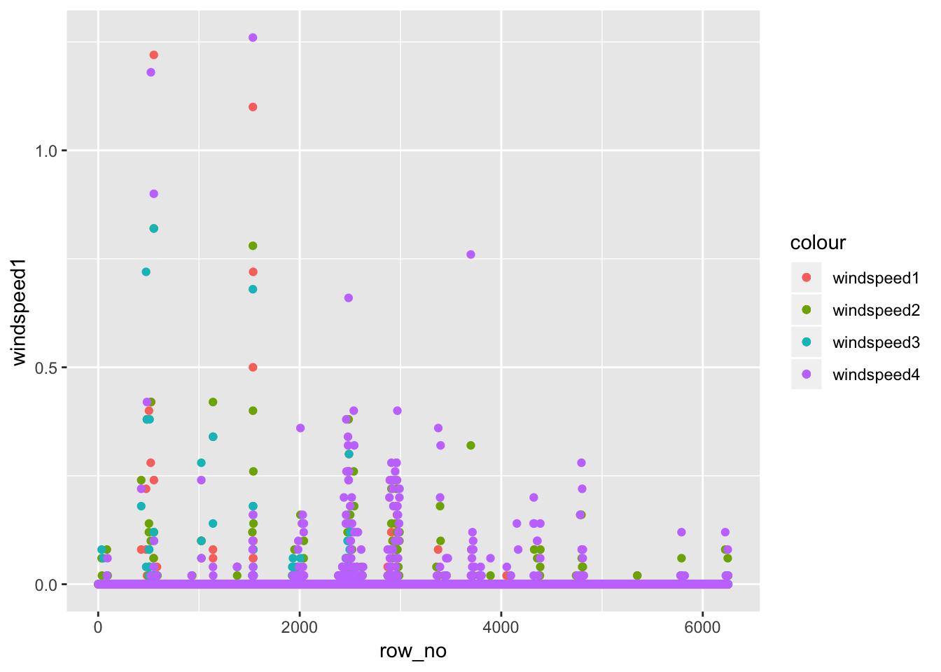
#ggplotly()Plot solar
av06_mm %>% dplyr::mutate(row_no= row_number()) %>% ggplot() +
geom_line(aes(row_no,solar,color='solar')) 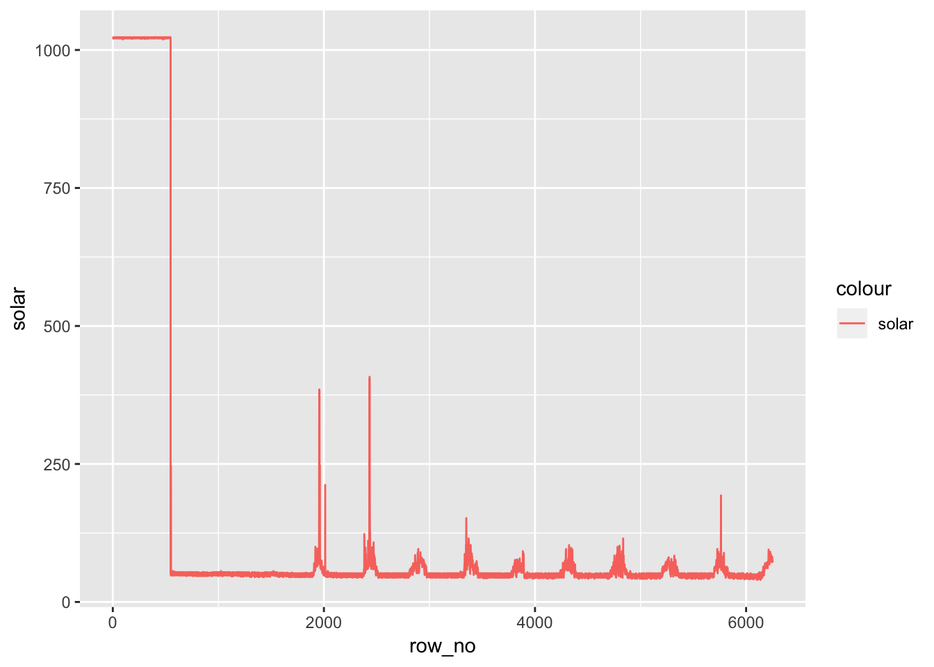
#ggplotly()Hourly temperature and precipitation (Pardise 5800) (vs Longmire station which is 2760 ft)
#Load a file
Paradise_2018<- read.csv('./data/Paradise_5400_feet_2018.csv')


Paradise_2018$date <- as.Date(Paradise_2018$Date.Time..PST., "%Y-%m-%d")
Paradise_2018$hr <-strftime(Paradise_2018$Date.Time..PST.,'%H')
Paradise_2018$min <-strftime(Paradise_2018$Date.Time..PST.,'%M')
Paradise_2018$month <- strftime(Paradise_2018$Date.Time..PST.,'%m')
Paradise_2018$Temperature..deg.C. <- (Paradise_2018$Temperature..deg.F. - 32) * (5/9)

Paradise_2018 %>% filter(month %in% c("09")) %>% ggplot(aes(date,Temperature..deg.C.)) +geom_point() + ggtitle("NWAC Temperature at Paradise(5400 ft)")+ xlab("Date") + ylab("Temp(Deg C)")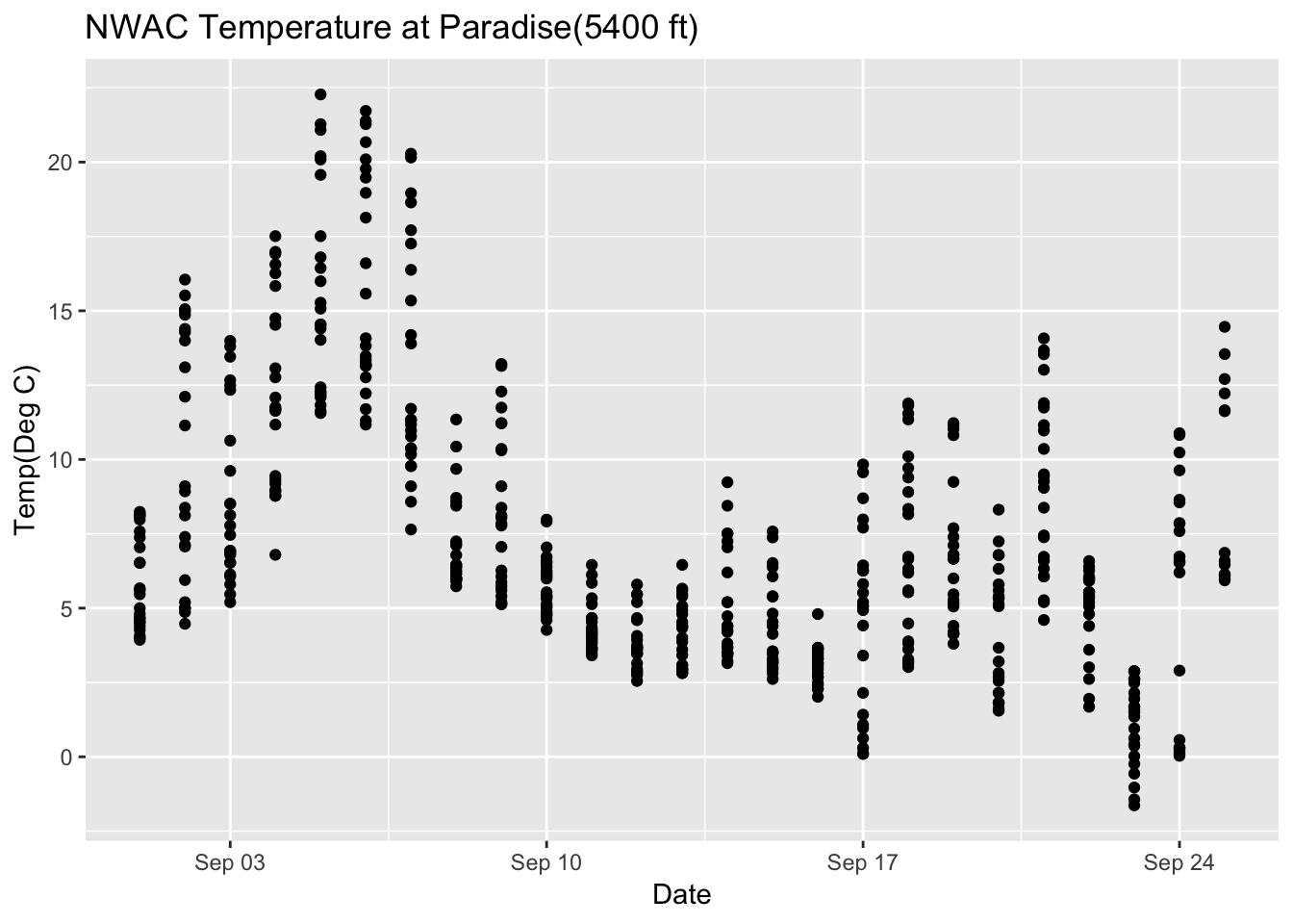
Extracting diurnal pattern for a day
Plot four wind along with other parameters
dp1<- av06_mm %>%  dplyr::mutate(row_no= row_number()) %>%  filter(row_no > 2292 & row_no < 2714) %>% ggplot() +
  geom_point(aes(row_no,windspeed1,color='windspeed1')) +
  geom_point(aes(row_no,windspeed2,color='windspeed2')) +
  geom_point(aes(row_no,windspeed3,color='windspeed3')) +
  geom_point(aes(row_no,windspeed4,color='windspeed4')) +
  geom_line(aes(row_no,log10(temp4),color='temp 4')) +
  geom_line(aes(row_no,log10(temp3),color='temp 3')) +
  geom_line(aes(row_no,log10(temp2),color='temp 2')) +
  geom_line(aes(row_no,log10(temp1),color='temp 1')) +
   geom_line(aes(row_no,log10(solar),color='solar'))
Trying smoothing to see the pattern
sp<- av06_mm %>%  dplyr::mutate(row_no= row_number()) %>%  filter(row_no > 2292 & row_no < 2714) %>% ggplot() +
  geom_point(aes(row_no,windspeed1,color='windspeed1')) + geom_smooth(aes(row_no,windspeed1),method='lm', se = FALSE)  +
  geom_point(aes(row_no,windspeed2,color='windspeed2')) + geom_smooth(aes(row_no,windspeed2),method='lm', se = FALSE)   +
  geom_smooth(aes(row_no,windspeed3,color='windspeed3')) + geom_smooth(aes(row_no,windspeed3),method='lm', se = FALSE)  +
  geom_smooth(aes(row_no,windspeed4,color='windspeed4')) + geom_smooth(aes(row_no,windspeed4),method='lm', se = FALSE)  +
  theme_classic()
#ggplotly(sp)
#api_create(sp, filename = "wind-profile-smoothed")
8.13 10-1-2018
With respect to microclimate measurements, forest canopy seems to be quite choppy(wind). Intuition says that there is so much buffering that a strong wind that has originated elsewhere when makes into canopies dissipates much quicker.
Feedback: a) not descernible wind profile, so quite hard to interpolate. b) temperature seems to be too low c) the temperatures at different heights should track each other.
8.14 Next steps
– Extract similiar segments and compare – How would a diurnation curve look like in the canopies at different heights ? – In open, my understanding so far, the temp closer to ground is warmer(much ?) in early hours of the day, but as the day warms, it flips i.e. the temp closer to ground is not that warm compared to higher heights(vertically). The air is much warmer at higher heights around solar max. Is this true ? Verify. Now, there could be exceptions, like inversion or cold air pooling.
8.15 10-2-2018
Microclim manuscript update.
Feedback : a) Show 2-3 days instead of whole week. b) The raster plot - it is still not clear on what is the difference ? c) remove the seasonal plot as daily variation should be sufficient.
Reflection:
8.16 10-17-2018
Feedback - Ideal would be to show multiple days plotted on the hourly x-axis to show the variation.
Typical weekly summer variation
decombined %>% filter(year(datec) %in% c(1981) & month(datec) %in% c(01) & day(datec) > 15 & day(datec) < 19)  %>%
  group_by(month,day,hr)  %>%
  ggplot() +
  geom_line(aes(hr,Tsurface-273.5,group=day,color=as.factor(day),linetype = 'Surface'),se=F)+     geom_line(aes(hr,TAH-273.5,group=day ,color=as.factor(day),linetype = 'Canopy'),se=F)+
  scale_colour_manual("Temperature on day", breaks = c("16", "17","18"), values = c("blue","red","green")) +
   scale_linetype_manual("Height",values=c("Surface"=2,"Canopy"=1)) +
  theme_minimal() + ggtitle("Variation in temperature at two different heights")  + xlab("Hour") +
  ylab("Temperature (°C)") + labs(colour = "Hour",
subtitle="1/16/81 - 1/18/81",caption="Data Source : http://www.microclim.org") 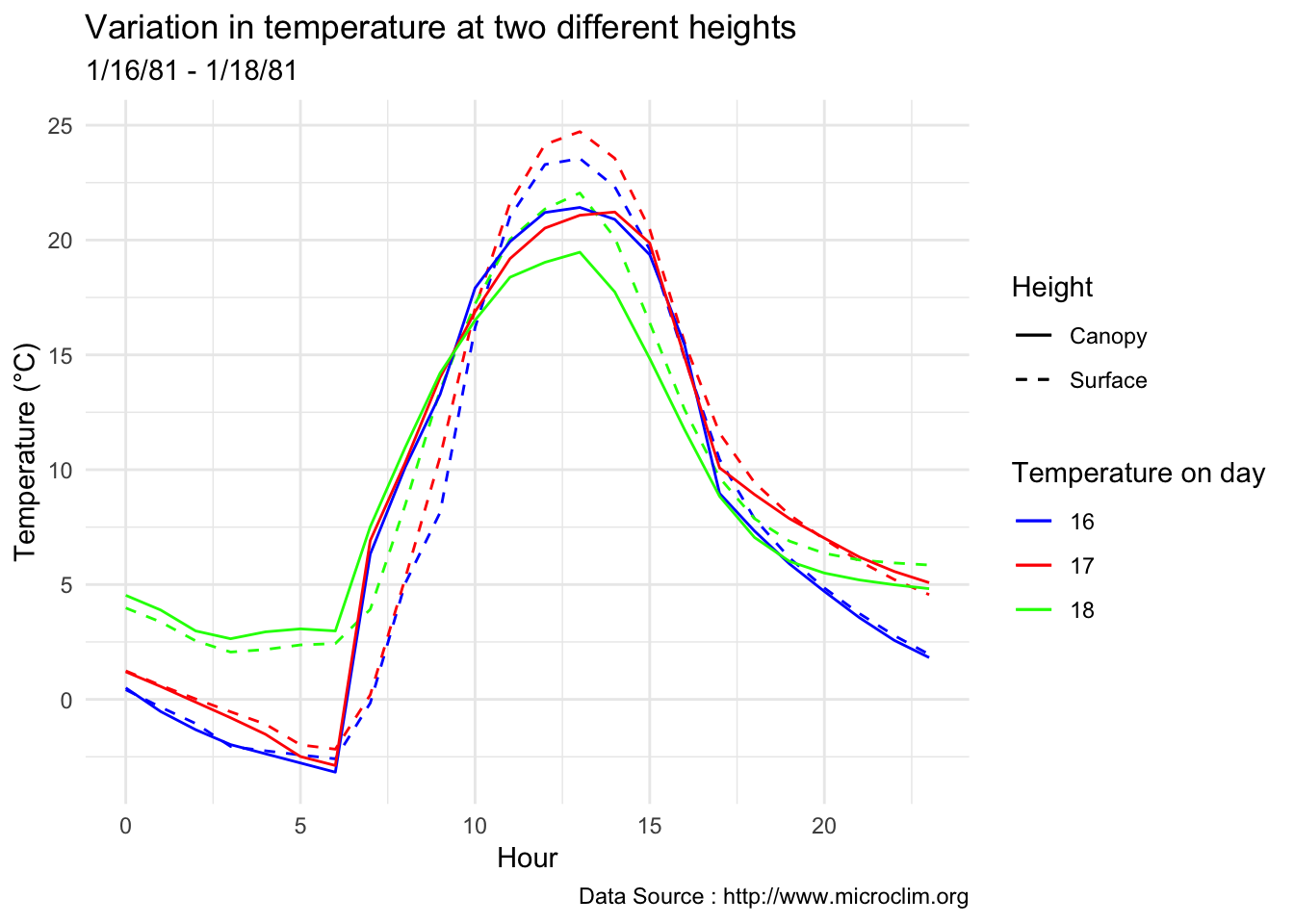
8.17 Open to-dos
– Take out the grid
Taking a shot at seasonal aspect of microclimate.
decombined %>% filter(year(datec) %in% c(1981) & month(datec) %in% c(06,07,08) )  %>%
  group_by(month,day,hr) %>% summarise(minST = min(Tsurface),minCT = min(TAH),maxST = max(Tsurface),maxCT = max(TAH)) %>%
  group_by(hr) %>% summarise(minST = mean(minST),minCT = mean(minCT),maxST = mean(maxST),maxCT = mean(maxCT)) %>%
  ggplot() +
  geom_line(aes(hr,minST-273.5,color='Surface Min'),linetype=1,se=F)+ geom_line(aes(hr,minCT-273.5,color='Canopy Min'),se=F)+
    geom_line(aes(hr,maxST-273.5,color='Surface Max'),se=F)+ geom_line(aes(hr,maxCT-273.5,color='Canopy Max'),se=F)+
  scale_colour_manual("Temperature at", breaks = c("Surface Min", "Canopy Min","Surface Max", "Canopy Max"), values = c("blue","red","green","pink")) +
  theme_minimal() + ggtitle("Summer trend of minimum temperature at different heights")  + xlab("Hour") +
  ylab("Temperature (°C)") + labs(colour = "Hour",
subtitle="Microclimate differences at two different heights",caption="Data Source : http://www.microclim.org") 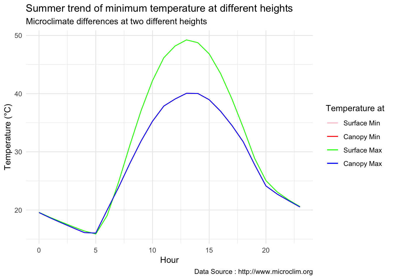
8.18 10-04-2018
Plot solar
av06_mm %>% mutate(row_no= row_number(),solarinunits= solar*1.76) %>% ggplot() +
geom_line(aes(row_no,solarinunits,color='solar')) 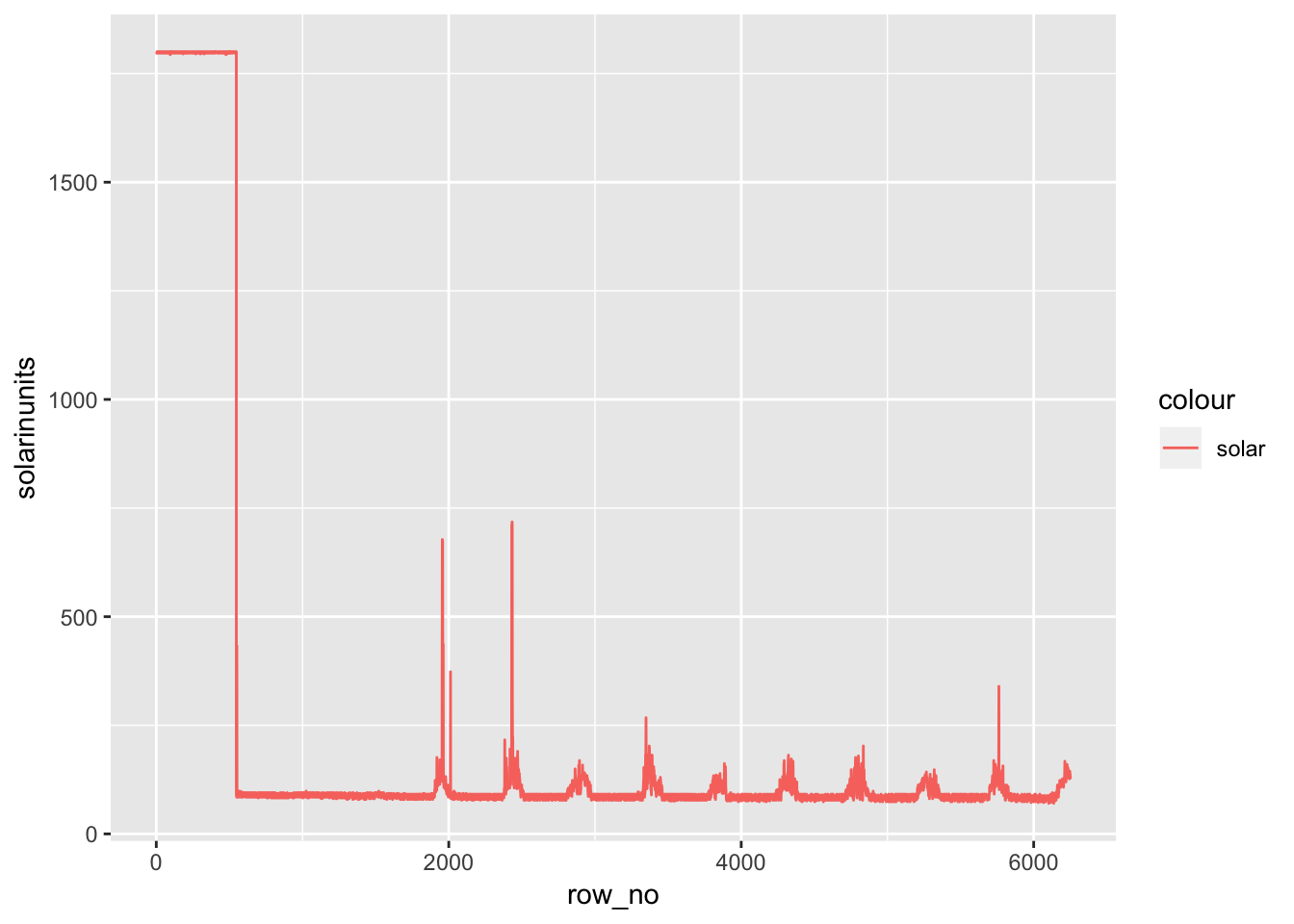
ggplotly()8.19 11-04-2018
Analysis of first set of data from the field.
Need to look at the hourly variation, we expect the ground to be cooler depending on the time of the day.
Lets look at one site
library(lubridate)
library(tidyverse)
mclim_AE10_TN01_2018<- read.csv('./data/DATALOG-AE10-TN01.CSV')
names(mclim_AE10_TN01_2018) <- c('time','nodeid','temp','batt')
mclim_AE10_TN01_2018$time <- as.POSIXct(mclim_AE10_TN01_2018$time, "%Y/%m/%d %H:%M:%S")

#Add hour month and day
## 11-05-2018
mclim_AE10_TN01_2018$hr <- hour(mclim_AE10_TN01_2018$time)
mclim_AE10_TN01_2018$minute<- minute(mclim_AE10_TN01_2018$time)
mclim_AE10_TN01_2018$day <- day(mclim_AE10_TN01_2018$time)
mclim_AE10_TN01_2018$month<- month(mclim_AE10_TN01_2018$time)

#Roughly one feet apart
mclim_AE10_TN01_2018$height <- 0

mclim_AE10_TN01_2018[mclim_AE10_TN01_2018$nodeid=='28244877910B0291' ,]$height <- 0.3
mclim_AE10_TN01_2018[mclim_AE10_TN01_2018$nodeid=='28A225779104022C' ,]$height <- 0.9
mclim_AE10_TN01_2018[mclim_AE10_TN01_2018$nodeid=='281D877791100268' ,]$height <- 0.6
mclim_AE10_TN01_2018[mclim_AE10_TN01_2018$nodeid=='282324779104023C' ,]$height <- 1.2

## Day plot , Representive day
mclim_AE10_TN01_2018 %>% filter(day(time) %in% '14' & !nodeid %in% c('282324779104023C')) %>%
ggplot( aes(time,temp,color = factor(height))) + geom_line() + theme_minimal() +
ggtitle("Variation in temperature at AE10 - Open")  + xlab("Date") +
  ylab("Temperature (°C)") + labs(colour = "Height(m)",
subtitle="9/17/2018",caption="Data Source : http://nanoclimate.org") 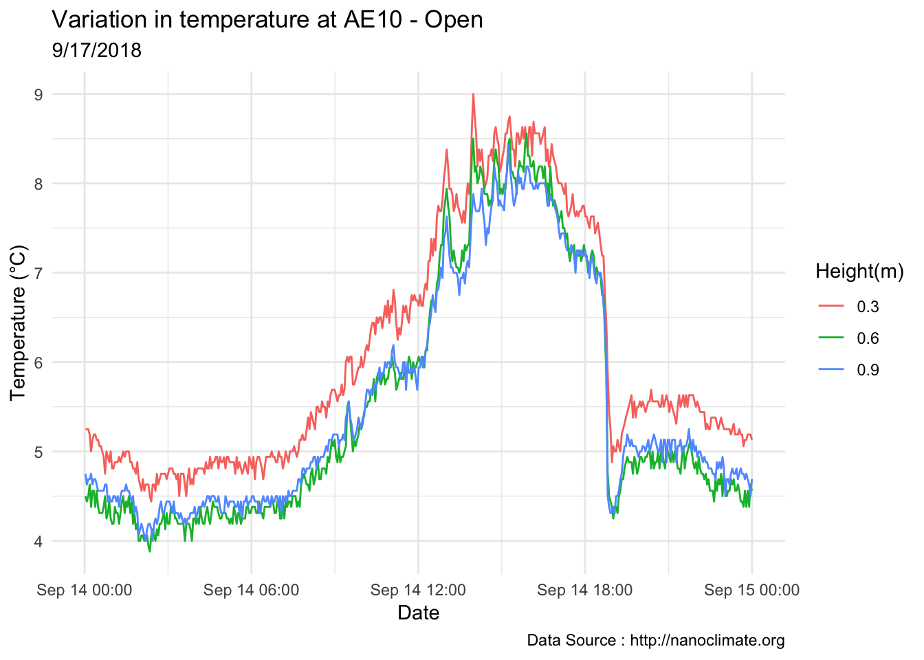
Do detailed variation
## Day plot , Representive day
mclim_AE10_TN01_2018 %>% filter(day(time) %in% '14' & !nodeid %in% c('282324779104023C')) %>%
ggplot( aes(time,temp,color = factor(height))) + geom_line() + theme_minimal() +
ggtitle("Variation in temperature at AE10 - Open - TN01")  + xlab("Date") +
  ylab("Temperature (°C)") + labs(colour = "Height(m)",
subtitle="9/17/2018",caption="Data Source : http://nanoclimate.org") 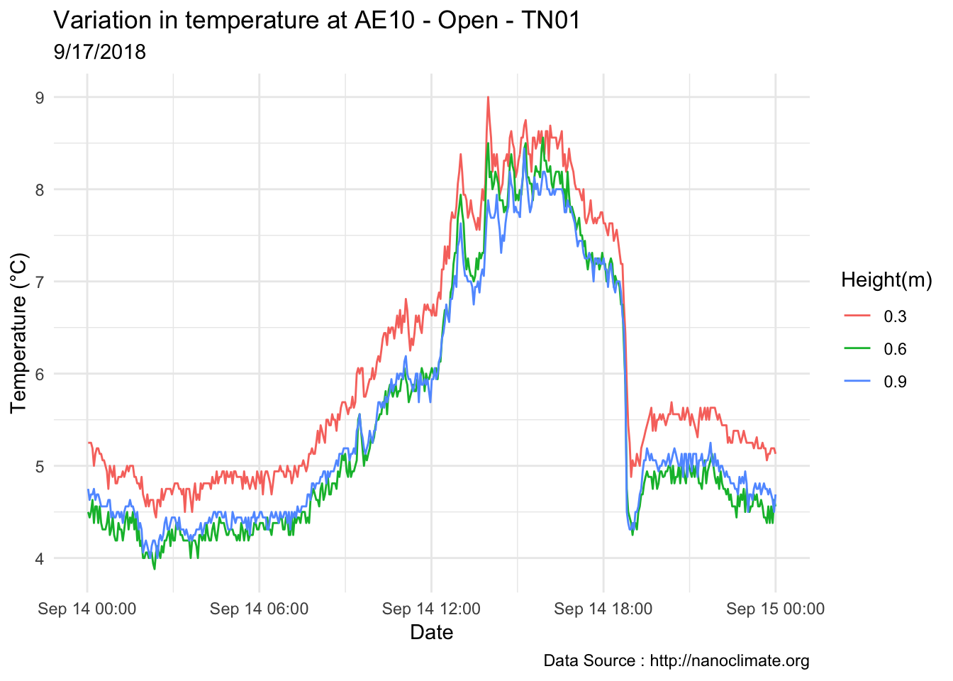
By minute
labelsx <- c( "0","12", "24", "36", "48" ,
             "1","12", "24", "36", "48",  "2" , "12", "24", "36", "48",
             "3", "12", "24", "36", "48",  "4",  "12", "24", "36", "48",
             "5", "12", "24", "36", "48",  "6",  "12", "24", "36", "48",
             "7", "12", "24", "36", "48", "8", "12", "24", "36", "48",
             "9", "12", "24", "36", "48", "10",  "12", "24", "36", "48",
             "11", "12", "24", "36", "48", "12",  "12", "24", "36", "48",
             "13", "12", "24", "36", "48", "14",  "12", "24", "36", "48",
             "15", "12", "24", "36", "48", "16",  "12", "24", "36", "48",
             "17", "12", "24", "36", "48", "18",  "12", "24", "36", "48",
             "19", "12", "24", "36", "48", "20",  "12", "24", "36", "48",
             "21", "12", "24", "36", "48", "22",  "12", "24", "36", "48",
             "23",  "12", "24", "36", "48")
## Day plot , Representive day
mclim_AE10_TN01_2018 %>%
    filter(day(time) %in% '14' & !height %in% c(1.2)  )  %>%
  group_by(height,hr,minute) %>%
  summarise(tempatmin = mean(temp)) %>%
    group_by(b = gl(ceiling(n()/4), 4, n())) %>%
group_by(height,hr,b) %>%
   summarize(heights = levels(as.factor(height)), meantemp = mean(tempatmin),
             sd = sd(tempatmin)) %>%
  mutate(newx= as.numeric(paste(hr,b,sep=""))) %>%  #select(newx) %>% distinct(newx)
  group_by(height) %>%
  mutate(index=1:n()) %>%
   ggplot() +
   geom_line(aes(index,meantemp,col=as.factor(height))) +
   #geom_line(data=paradise[paradise$day==14,], aes(hour,temp,col='Reference')) +
    labs(x="Hour", y="Temperature (°C)", tag="(g)",colour = "Height (m)") +
   theme_minimal() +
  scale_x_continuous(breaks = seq(0,119,by=1), limits = c(0,120),labels = labelsx) +
   theme( panel.grid.major = element_blank(),

        legend.position = c(.2,.9),
         legend.title=element_text(size=9),
         legend.text=element_text(size=8),
         legend.background = element_rect(color = "grey90",
                                          size = .5, linetype = "dashed"),
         axis.text.x=element_text(angle=90, hjust=0)) +
   theme(strip.text.x = element_text(face="bold", size=4)) +
   theme(strip.text.y = element_text(face="bold", size=8))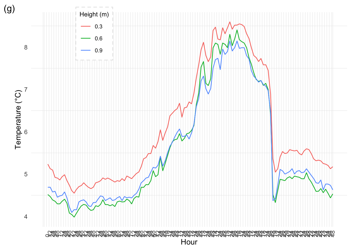
Lets look at a closed site
mclim_AE10_TN02_2018<- read.csv('./data/DATALOG-AE10-TN02.CSV')
names(mclim_AE10_TN02_2018) <- c('time','nodeid','temp','batt')
mclim_AE10_TN02_2018$time <- as.POSIXct(mclim_AE10_TN02_2018$time, "%Y/%m/%d %H:%M:%S")

#Add hour month and day
## 11-05-2018
mclim_AE10_TN02_2018$hr <- hour(mclim_AE10_TN02_2018$time)
mclim_AE10_TN02_2018$minute <- minute(mclim_AE10_TN02_2018$time)
mclim_AE10_TN02_2018$day <- day(mclim_AE10_TN02_2018$time)
mclim_AE10_TN02_2018$month<- month(mclim_AE10_TN02_2018$time)

#Roughly one feet apart
mclim_AE10_TN02_2018$height <- 0

mclim_AE10_TN02_2018[mclim_AE10_TN02_2018$nodeid=='2862367791040281' ,]$height <- 1.2
mclim_AE10_TN02_2018[mclim_AE10_TN02_2018$nodeid=='286E9D77910802F2' ,]$height <- 0.6
mclim_AE10_TN02_2018[mclim_AE10_TN02_2018$nodeid=='28A91B7791060263' ,]$height <- 0.3
mclim_AE10_TN02_2018[mclim_AE10_TN02_2018$nodeid=='280704779106023F' ,]$height <- 0.9

## Day plot , Representive day
mclim_AE10_TN02_2018 %>% filter(day(time) %in% '14' ) %>%
ggplot( aes(time,temp,color = factor(height))) + geom_line() + theme_minimal() +
ggtitle("Variation in temperature at AE10 - Closed - TN02")  + xlab("Date") +
  ylab("Temperature (°C)") + labs(colour = "Height(m)",
subtitle="9/14/2018",caption="Data Source : http://nanoclimate.org") 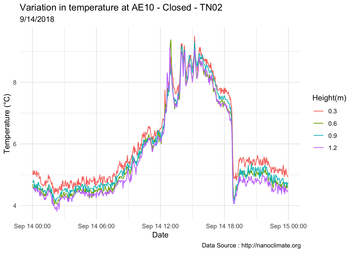
Lets look at another site
mclim_AE10_TN03_2018<- read.csv('./data/DATALOG-AE10-TN03.CSV')
names(mclim_AE10_TN03_2018) <- c('time','nodeid','temp','batt')
mclim_AE10_TN03_2018$time <- as.POSIXct(mclim_AE10_TN03_2018$time, "%Y/%m/%d %H:%M:%S")

#Add hour month and day
## 11-05-2018
mclim_AE10_TN03_2018$hr <- hour(mclim_AE10_TN03_2018$time)
mclim_AE10_TN03_2018$day <- day(mclim_AE10_TN03_2018$time)
mclim_AE10_TN03_2018$month<- month(mclim_AE10_TN03_2018$time)
mclim_AE10_TN03_2018$minute<- minute(mclim_AE10_TN03_2018$time)
#Roughly one feet apart
mclim_AE10_TN03_2018$height <- 0

mclim_AE10_TN03_2018[mclim_AE10_TN03_2018$nodeid=='28BF3D77910B0267' ,]$height <- 1.2
mclim_AE10_TN03_2018[mclim_AE10_TN03_2018$nodeid=='28CCF877910A0292' ,]$height <- 0.6
mclim_AE10_TN03_2018[mclim_AE10_TN03_2018$nodeid=='283C8E7791080280' ,]$height <- 0.3
mclim_AE10_TN03_2018[mclim_AE10_TN03_2018$nodeid=='28E210779104020F' ,]$height <- 0.9

## Day plot , Representive day
mclim_AE10_TN03_2018 %>% filter(day(time) %in% '14' ) %>%
ggplot( aes(time,temp,color = factor(height))) + geom_line() + theme_minimal() +
ggtitle("Variation in temperature at AE10 - Closed - TN03")  + xlab("Date") +
  ylab("Temperature (°C)") + labs(colour = "Height(m)",
subtitle="9/14/2018",caption="Data Source : http://nanoclimate.org") 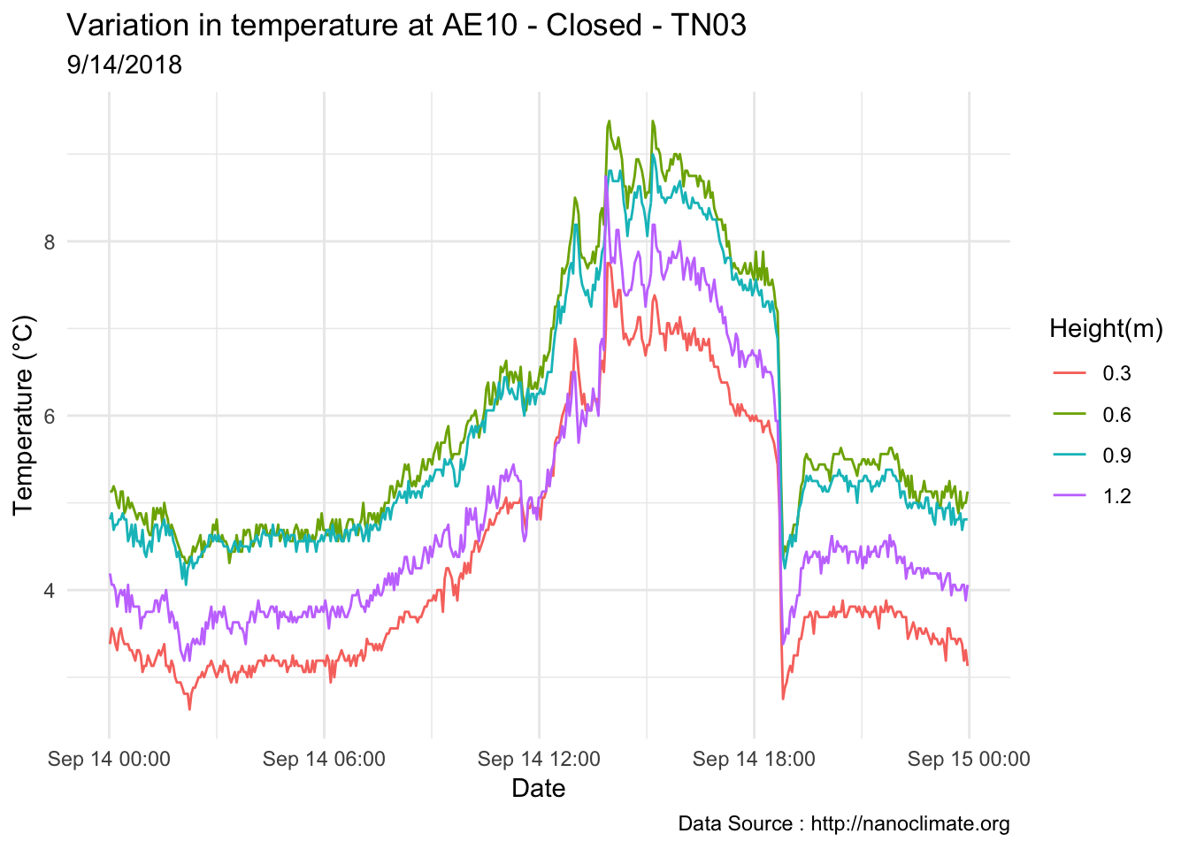
Lets look at the Anemometer site
mclim_AE10_CN01_2018<-read_csv('./data/DATALOG-AE10-CN01.CSV')## Parsed with column specification:
## cols(
## date = col_character(),
## temp1 = col_double(),
## temp2 = col_double(),
## temp3 = col_double(),
## temp4 = col_double(),
## windspeed1 = col_double(),
## windspeed2 = col_double(),
## windspeed3 = col_double(),
## windspeed4 = col_double(),
## winddirection1 = col_double(),
## winddirection2 = col_double(),
## winddirection3 = col_double(),
## winddirection4 = col_double(),
## solar = col_double(),
## battery = col_double()
## )#mclim_AE10_CN01_2018<- read.csv('./data/DATALOG-AE10-CN01.CSV',stringsAsFactors = T)
names(mclim_AE10_CN01_2018)## [1] "date" "temp1" "temp2" "temp3"
## [5] "temp4" "windspeed1" "windspeed2" "windspeed3"
## [9] "windspeed4" "winddirection1" "winddirection2" "winddirection3"
## [13] "winddirection4" "solar" "battery"mclim_AE10_CN01_2018$time <- as_datetime(mclim_AE10_CN01_2018$date, format="%m/%d/%y %H:%M:%S",tz="America/Los_Angeles")
mclim_AE10_CN01_2018$time <-as.POSIXct(mclim_AE10_CN01_2018$time)
#Add hour month and day
## 11-05-2018
mclim_AE10_CN01_2018$hr <- hour(mclim_AE10_CN01_2018$time)
mclim_AE10_CN01_2018$day <- day(mclim_AE10_CN01_2018$time)
mclim_AE10_CN01_2018$month<- month(mclim_AE10_CN01_2018$time)
#Roughly one feet apart
mclim_AE10_CN01_2018$height <- 0
#therm1,28782877910A0217 - 0.6
#therm2,284CCE7791090235 - 1.2
#therm3,286C7A7791080217 - 0.9
#therm4,280A2577910A020D - 0.3
# mclim_AE10_CN01_2018[mclim_AE10_CN01_2018$nodeid=='2862367791040281' ,]$height <- 1.2
# mclim_AE10_CN01_2018[mclim_AE10_CN01_2018$nodeid=='286E9D77910802F2' ,]$height <- 0.6
# mclim_AE10_CN01_2018[mclim_AE10_CN01_2018$nodeid=='28A91B7791060263' ,]$height <- 0.3
# mclim_AE10_CN01_2018[mclim_AE10_CN01_2018$nodeid=='280704779106023F' ,]$height <- 0.9
## Day plot , Representive day
mclim_AE10_CN01_2018 %>% filter(month %in% c(9) & day(time) %in% '14' ) %>%
ggplot() + geom_line( aes(time,temp1,color = '0.6')) +
geom_line( aes(time,temp2,color = '1.2')) +
geom_line( aes(time,temp3,color = '0.9')) +
geom_line( aes(time,temp4,color = '0.3')) +
theme_classic() +
ggtitle("Variation in temperature at AE10 w/Wind - Open") + xlab("Date") +
ylab("Temperature (°C)") + labs(colour = "Height(m)",
subtitle="9/14/2018",caption="Data Source : http://nanoclimate.org") 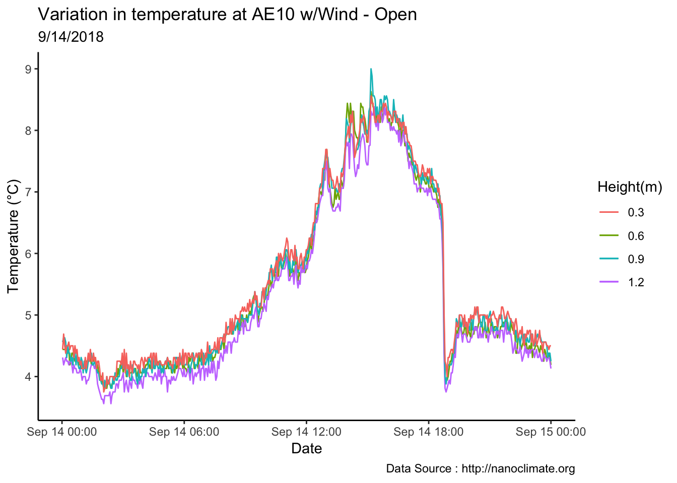
By day with wind
mclim_AE10_CN01_2018 %>% filter(month %in% c(9) ) %>%
ggplot() + geom_line( aes(time,temp1,color = '0.6')) +
geom_line( aes(time,temp2,color = '1.2')) +
geom_line( aes(time,temp3,color = '0.9')) +
geom_line( aes(time,temp4,color = '0.3')) +
theme_minimal() +
ggtitle("Variation in temperature at AE10 w/Wind - Open") + xlab("Date") +
ylab("Temperature (°C)") + labs(colour = "Height(m)",
subtitle="Microclimate profiles",caption="Data Source : http://nanoclimate.org") 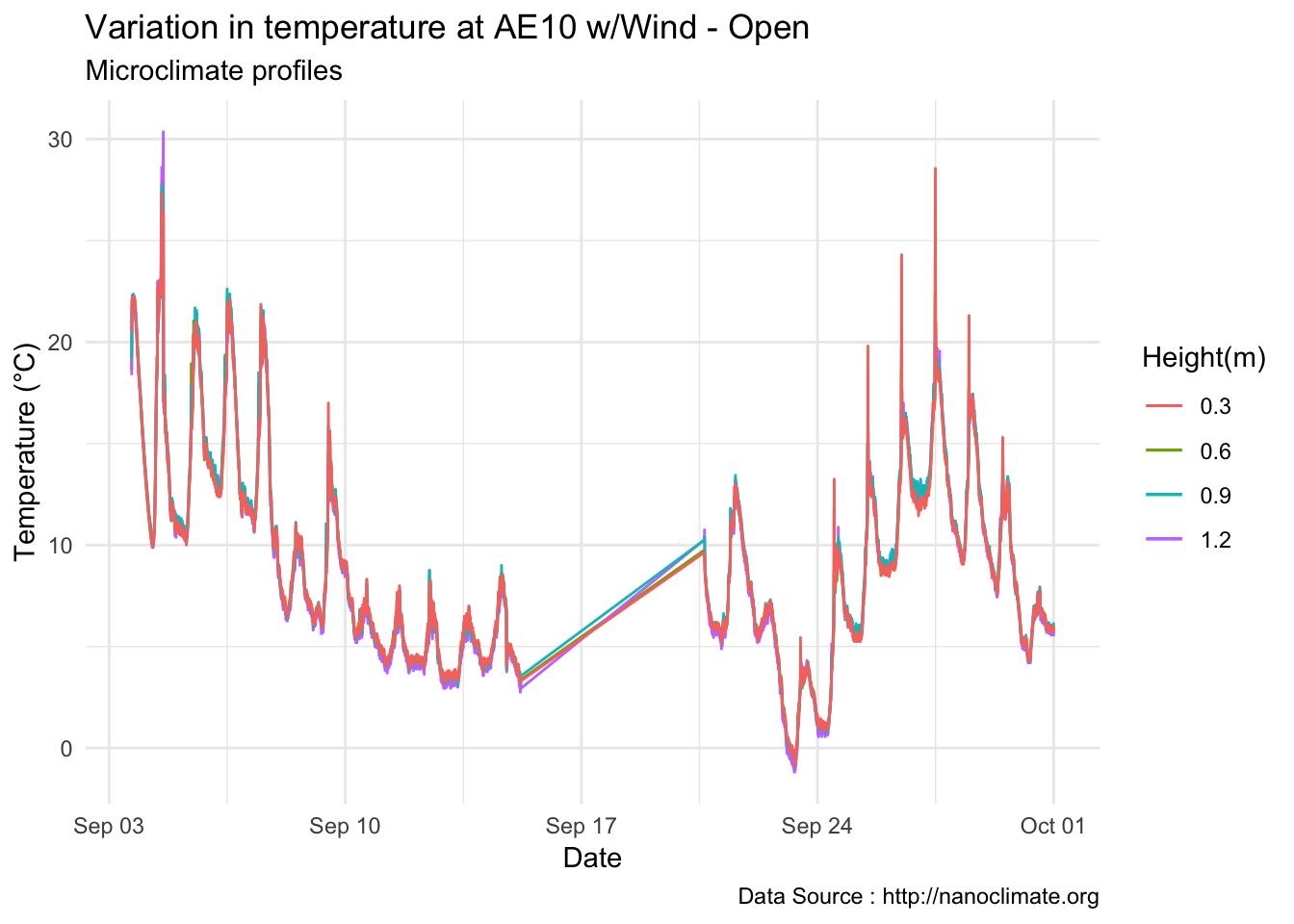 By day with wind
mclim_AE10_TN01_2018 %>% filter(!nodeid %in% c('282324779104023C') & temp >0 ) %>%
ggplot( aes(time,temp,color = factor(height))) + geom_line() + theme_minimal() +
ggtitle("Variation in temperature at AE10 - Open")  + xlab("Date") +
  ylab("Temperature (°C)") + labs(colour = "Height(m)",
subtitle="Microclimate profiles",caption="Data Source : http://nanoclimate.org") 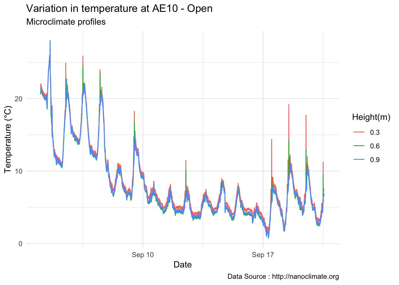
Wind ptrofiles
mclim_AE10_CN01_2018<-read_csv('./data/DATALOG-AE10-CN01.CSV')## Parsed with column specification:
## cols(
## date = col_character(),
## temp1 = col_double(),
## temp2 = col_double(),
## temp3 = col_double(),
## temp4 = col_double(),
## windspeed1 = col_double(),
## windspeed2 = col_double(),
## windspeed3 = col_double(),
## windspeed4 = col_double(),
## winddirection1 = col_double(),
## winddirection2 = col_double(),
## winddirection3 = col_double(),
## winddirection4 = col_double(),
## solar = col_double(),
## battery = col_double()
## )#mclim_AE10_CN01_2018<- read.csv('./data/DATALOG-AE10-CN01.CSV',stringsAsFactors = T)
names(mclim_AE10_CN01_2018)## [1] "date" "temp1" "temp2" "temp3"
## [5] "temp4" "windspeed1" "windspeed2" "windspeed3"
## [9] "windspeed4" "winddirection1" "winddirection2" "winddirection3"
## [13] "winddirection4" "solar" "battery"mclim_AE10_CN01_2018$time <- as_datetime(mclim_AE10_CN01_2018$date, format="%m/%d/%y %H:%M:%S",tz="America/Los_Angeles")
mclim_AE10_CN01_2018$time <-as.POSIXct(mclim_AE10_CN01_2018$time)
#Add hour month and day
## 11-05-2018
mclim_AE10_CN01_2018$hr <- hour(mclim_AE10_CN01_2018$time)
mclim_AE10_CN01_2018$minute <- minute(mclim_AE10_CN01_2018$time)
mclim_AE10_CN01_2018$day <- day(mclim_AE10_CN01_2018$time)
mclim_AE10_CN01_2018$month<- month(mclim_AE10_CN01_2018$time)
#Roughly one feet apart
mclim_AE10_CN01_2018$height <- 0
#therm1,28782877910A0217 - 0.6
#therm2,284CCE7791090235 - 1.2
#therm3,286C7A7791080217 - 0.9
#therm4,280A2577910A020D - 0.3
# mclim_AE10_CN01_2018[mclim_AE10_CN01_2018$nodeid=='2862367791040281' ,]$height <- 1.2
# mclim_AE10_CN01_2018[mclim_AE10_CN01_2018$nodeid=='286E9D77910802F2' ,]$height <- 0.6
# mclim_AE10_CN01_2018[mclim_AE10_CN01_2018$nodeid=='28A91B7791060263' ,]$height <- 0.3
# mclim_AE10_CN01_2018[mclim_AE10_CN01_2018$nodeid=='280704779106023F' ,]$height <- 0.9
## Day plot , Representive day
mclim_AE10_CN01_2018 %>% filter(month %in% c(9) & day(time) %in% '14' & hr %in% c(13,14,15,16,17,18,19)) %>%
ggplot() + geom_line( aes(time,windspeed1,color = '0.6')) +
geom_line( aes(time,windspeed2,color = '1.2')) +
geom_line( aes(time,windspeed3,color = '0.9')) +
geom_line( aes(time,windspeed4,color = '0.3')) +
theme_minimal() +
ggtitle("Variation in wind at AE10 w/Wind - Open") + xlab("Date") +
ylab("Wind (km/hr)") + labs(colour = "Height(m)",
subtitle="9/14/2018",caption="Data Source : http://nanoclimate.org") 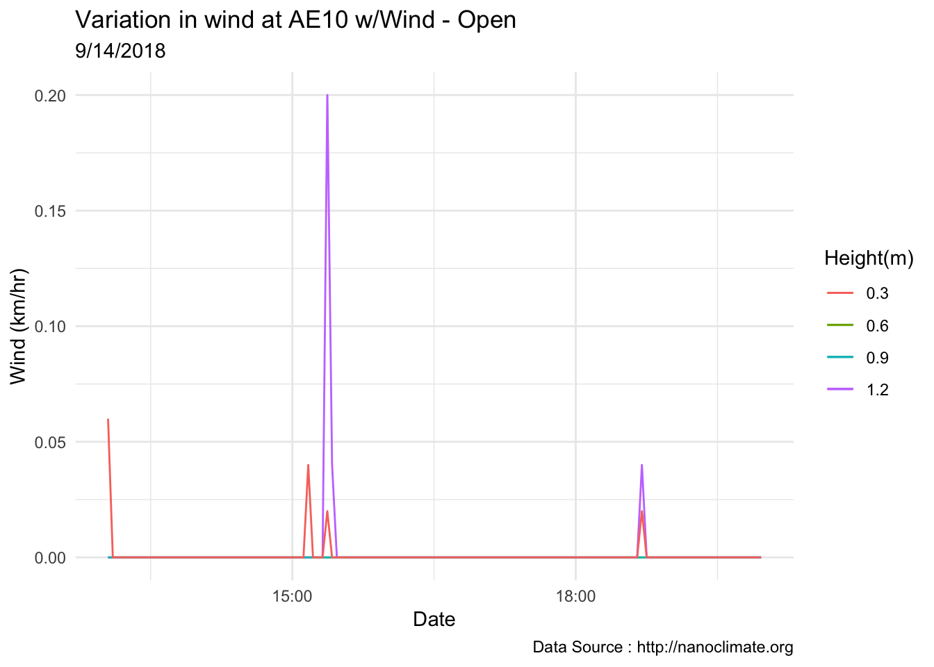
mclim_AE10_CN01_2018 %>% filter (month %in% c(9) ) %>% group_by(month,day) %>%
summarize(maxtemp = max(temp1),mintemp = min(temp1)) %>% ggplot() + geom_line(aes(day,maxtemp,col='red')) +
geom_line(aes(as.numeric(day),mintemp,col='blue')) +
theme_classic() + labs(x="Day", y="Temperature(°C) ",subtitle="Microclimate station - AE10 - 2018/9 ", caption="Data Source : http://nanoclimate.org") +
geom_hline(aes(yintercept=9),colour="black", linetype="dashed") +
scale_colour_manual(name = 'Temperature',
values =c('red'='red','blue'='blue'), labels = c('Max','Min'))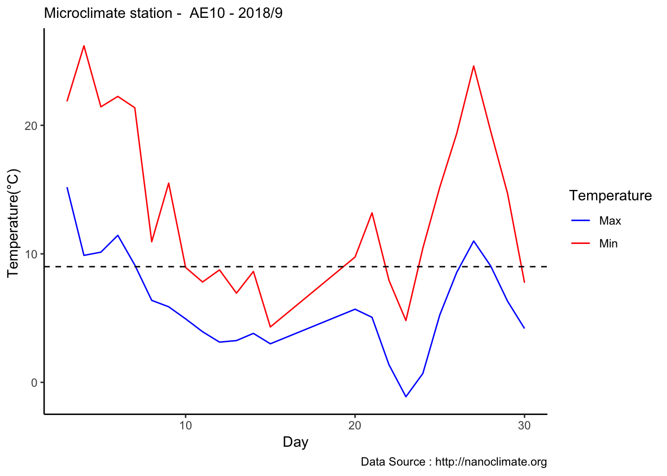 Diel
Diel
mclim_AE10_CN01_2018 %>% filter (month %in% c(9) ) %>% group_by(month,day) %>%
   summarize(maxtemp = max(temp1),mintemp = min(temp1)) %>% ggplot() +
  geom_line(aes(as.numeric(day),maxtemp-mintemp,col='red')) +
   theme_classic() + labs(x="Day", y="Temperature(°C) ",subtitle="Microclimate station -  AE10 - 2018/9 ",                                                                                                   caption="Data Source : http://nanoclimate.org") +
   geom_hline(aes(yintercept=9),colour="black", linetype="dashed")  +
    scale_colour_manual(name = 'Diel variation',
         values =c('red'='red'), labels = c('Diurnal'))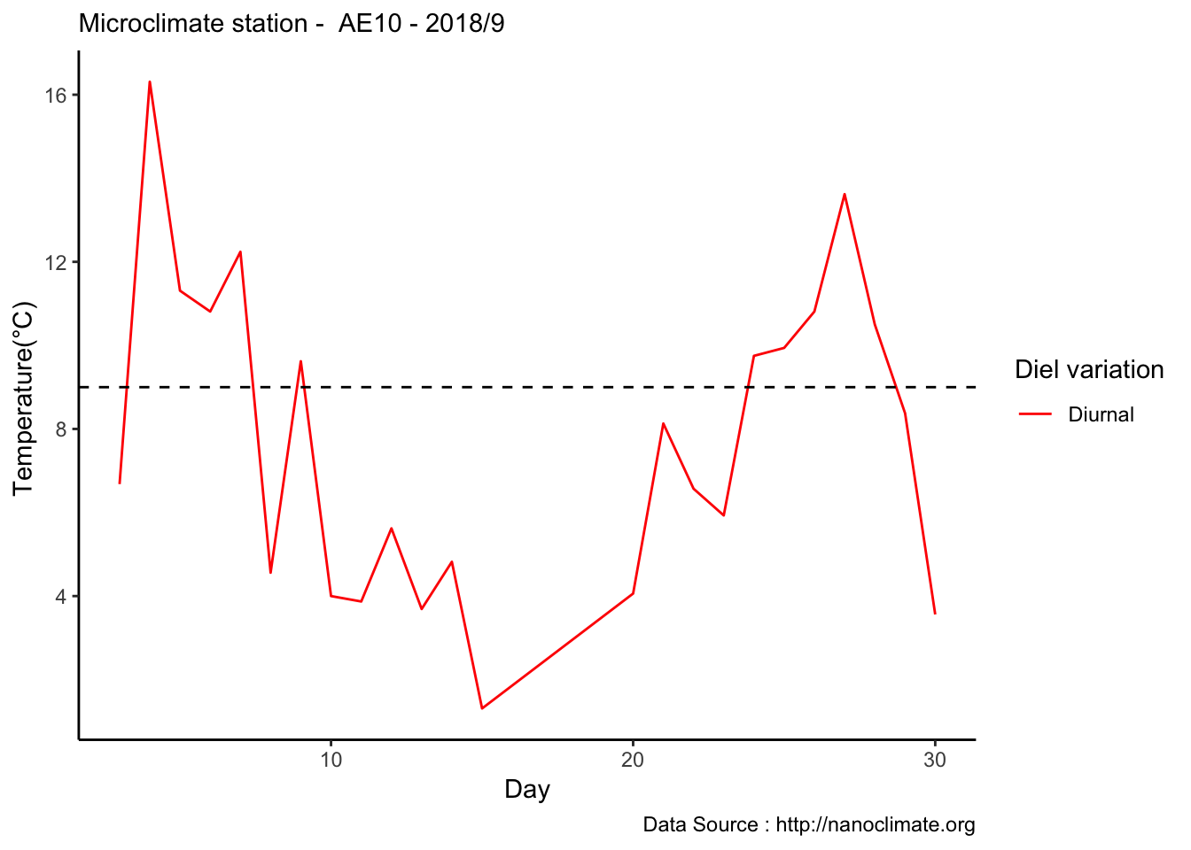
Diel by hour
mclim_AE10_CN01_2018 %>% filter (!is.na(mclim_AE10_CN01_2018$minute) & month %in% c(9) ) %>% group_by(month,day,hr) %>%
   summarize(meantemp1 = mean(temp1),meantemp2 = mean(temp2),meantemp3 = mean(temp3),meantemp4 = mean(temp4)) %>%
  group_by(hr) %>%
  ggplot() +
  geom_smooth(aes(as.numeric(hr),meantemp1,col='red'),se = F) +
  geom_smooth(aes(as.numeric(hr),meantemp2,col='blue'),se = F) +
  geom_smooth(aes(as.numeric(hr),meantemp3,col='green'),se = F) +
  geom_smooth(aes(as.numeric(hr),meantemp4,col='purple'),se = F) +
   theme_classic() + labs(x="Hour", y="Temperature(°C) ",subtitle="Microclimate station -  AE10 - 2018/9 ",                                                                                                   caption="Data Source : http://nanoclimate.org") +
   geom_hline(aes(yintercept=9),colour="black", linetype="dashed")  +
    scale_colour_manual(name = 'Heights',
         values =c('red'='red','blue'='blue','green'='green','purple'='purple'), labels = c('1.2','.9','.6','.3'))
## `geom_smooth()` using method = 'loess' and formula 'y ~ x'
## `geom_smooth()` using method = 'loess' and formula 'y ~ x'
## `geom_smooth()` using method = 'loess' and formula 'y ~ x'
## `geom_smooth()` using method = 'loess' and formula 'y ~ x'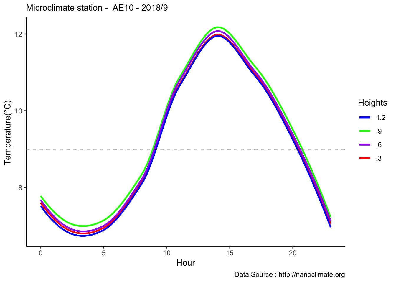
Diel does not make sense
mclim_AE10_CN01_2018 %>% filter (!is.na(mclim_AE10_CN01_2018$minute) & month %in% c(9) ) %>% group_by(month,day,hr,minute) %>%
  summarise(m1= mean(temp1),m2= mean(temp2),m3= mean(temp3),m4= mean(temp4)) %>%
   mutate(dh1 = mean(min(m1) - max(m1)) ,dh2 = mean(min(m2) - max(m2)),dh3 = mean(min(m3) - max(m3)),dh4 = mean(min(m4) - max(m4))) %>%
  group_by(hr) %>%
  ggplot() +
  geom_smooth(aes(as.numeric(hr),dh1,col='red'),se = F) +
  geom_smooth(aes(as.numeric(hr),dh2,col='blue'),se = F) +
  geom_smooth(aes(as.numeric(hr),dh3,col='green'),se = F) +
  geom_smooth(aes(as.numeric(hr),dh4,col='purple'),se = F) +
   theme_classic() + labs(x="Hour", y="Temperature(°C) ",subtitle="Microclimate station -  AE10 - 2018/9 ",                                                                                                   caption="Data Source : http://nanoclimate.org") +
   geom_hline(aes(yintercept=9),colour="black", linetype="dashed")  +
    scale_colour_manual(name = 'Heights',
         values =c('red'='red','blue'='blue','green'='green','purple'='purple'), labels = c('1.2','.9','.6','.3'))
## `geom_smooth()` using method = 'gam' and formula 'y ~ s(x, bs = "cs")'
## `geom_smooth()` using method = 'gam' and formula 'y ~ s(x, bs = "cs")'
## `geom_smooth()` using method = 'gam' and formula 'y ~ s(x, bs = "cs")'
## `geom_smooth()` using method = 'gam' and formula 'y ~ s(x, bs = "cs")'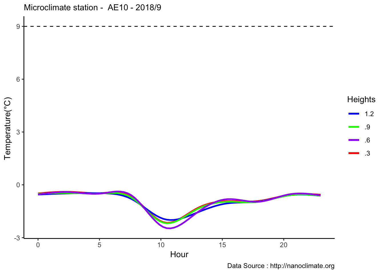
Diel does not make sense
mclim_AE10_CN01_2018 %>% filter (!is.na(mclim_AE10_CN01_2018$minute) & month %in% c(9) ) %>%
group_by(month,day,hr) %>%
summarise(m1= mean(temp1),m2= mean(temp2),m3= mean(temp3),m4= mean(temp4)) %>%
group_by(hr) %>%
summarise(m1= mean(m1),m2= mean(m2),m3= mean(m3),m4= mean(m4)) %>%
ggplot() +
geom_line(aes(as.numeric(hr),m1,col='1')) +
geom_line(aes(as.numeric(hr),m2,col='2')) +
geom_line(aes(as.numeric(hr),m3,col='3')) +
geom_line(aes(as.numeric(hr),m4,col='4')) +
theme_classic() + labs(x="Hour", y="Temperature(°C) ",subtitle="Microclimate station - AE10 - September 2018 ", caption="Data Source : http://nanoclimate.org") +
geom_hline(aes(yintercept=9),colour="black", linetype="dashed") +
scale_colour_manual(name = 'Diurnal variation at heights (m)',
values =c('1'='red','2'='blue','3'='green','4'='purple'), labels = c('1.2','.9','.6','.3'))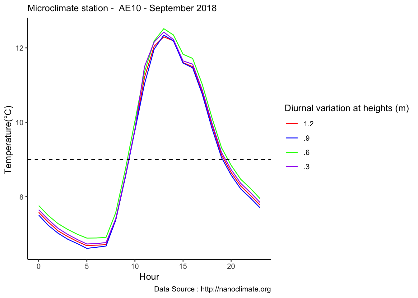 Lapse rate calculator
https://www.shodor.org/os411/courses/_master/tools/calculators/lapserate/
8.20 11-19-2018
Few days in September (Late September)
mclim_AE10_CN01_2018 %>% filter (!is.na(mclim_AE10_CN01_2018$minute) & month %in% c(9) ) %>%
filter( day > 20 & day < 24) %>%
group_by(month,day,hr) %>%
summarise(m1= mean(temp1),m2= mean(temp2),m3= mean(temp3),m4= mean(temp4)) %>%
group_by(day,hr) %>%
ggplot() +
geom_line(aes(hr,m1,group=day,color=as.factor(day),linetype = '0.3'),se=F)+
geom_line(aes(hr,m4,group=day ,color=as.factor(day),linetype = '1.2'),se=F)+
scale_colour_manual("Temperature on day", breaks = c("21", "22","23"), values = c("blue","red","green")) +
scale_linetype_manual("Height(m)",values=c("0.3"=2,"1.2"=1)) +
theme_classic() + ggtitle("Variation in temperature at two different heights at AE10") + xlab("Hour") +
ylab("Temperature (°C)") + labs(colour = "Hour",
subtitle="9/21/18 - 9/23/19",caption="Data Source : http://www.nanoclimate.org") 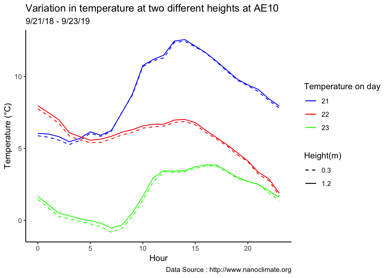 Early in the month
mclim_AE10_CN01_2018 %>%  filter (!is.na(mclim_AE10_CN01_2018$minute) & month %in% c(9) ) %>%
  filter( day > 11 & day < 15)  %>%
    group_by(month,day,hr) %>%
    summarise(m1= mean(temp1),m2= mean(temp2),m3= mean(temp3),m4= mean(temp4)) %>%
  group_by(day,hr) %>%
  ggplot() +
  geom_line(aes(hr,m1,group=day,color=as.factor(day),linetype = '0.3'),se=F)+
  geom_line(aes(hr,m4,group=day ,color=as.factor(day),linetype = '1.2'),se=F)+
  scale_colour_manual("Temperature on day", breaks = c("12", "13","14"), values = c("blue","red","green")) +
   scale_linetype_manual("Height(m)",values=c("0.3"=2,"1.2"=1)) +
  theme_classic()  + ggtitle("Variation in temperature at two different heights at AE10")  + xlab("Hour") +
  ylab("Temperature (°C)") + labs(colour = "Hour",
                                subtitle="9/12/18 - 9/14/19",caption="Data Source : http://www.nanoclimate.org")
Minute resolution
Early in the month
mclim_AE10_CN01_2018 %>%  filter (!is.na(mclim_AE10_CN01_2018$minute) & month %in% c(9) ) %>%
  filter( day > 11 & day < 15)  %>%
    group_by(month,day,hr) %>%
    add_count(wt=3) %>%
    summarise(m1= mean(temp1),m2= mean(temp2),m3= mean(temp3),m4= mean(temp4)) %>%
  group_by(day,hr) %>%
  ggplot() +
  geom_line(aes(hr,m1,group=day,color=as.factor(day),linetype = '0.3'),se=F)+
  geom_line(aes(hr,m4,group=day ,color=as.factor(day),linetype = '1.2'),se=F)+
  scale_colour_manual("Temperature on day", breaks = c("12", "13","14"), values = c("blue","red","green")) +
   scale_linetype_manual("Height(m)",values=c("0.3"=2,"1.2"=1)) +
  theme_classic()  + ggtitle("Variation in temperature at two different heights at AE10")  + xlab("Hour") +
  ylab("Temperature (°C)") + labs(colour = "Hour",
subtitle="9/12/18 - 9/14/19",caption="Data Source : http://www.nanoclimate.org") 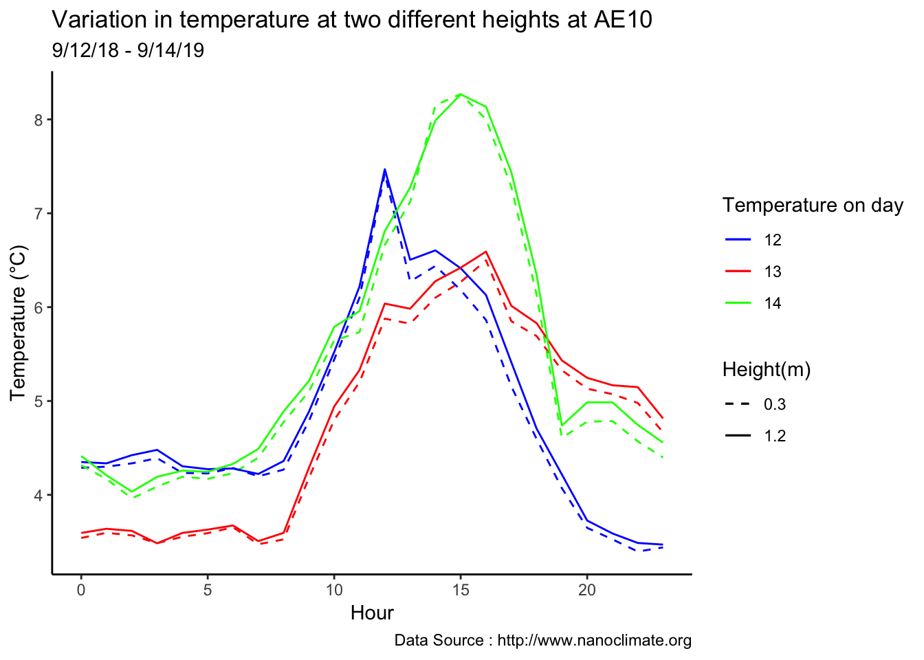
Minute resolution
Early in the month
mclim_AE10_CN01_2018$segment <- 0
mclim_AE10_CN01_2018[!is.na(mclim_AE10_CN01_2018$minute) & mclim_AE10_CN01_2018$minute >0 & mclim_AE10_CN01_2018$minute <=15  ,]$segment <- 1
mclim_AE10_CN01_2018[!is.na(mclim_AE10_CN01_2018$minute) & mclim_AE10_CN01_2018$minute >15 & mclim_AE10_CN01_2018$minute <=30  ,]$segment <- 2
mclim_AE10_CN01_2018[!is.na(mclim_AE10_CN01_2018$minute) & mclim_AE10_CN01_2018$minute >30 & mclim_AE10_CN01_2018$minute <=45  ,]$segment <- 3
mclim_AE10_CN01_2018[!is.na(mclim_AE10_CN01_2018$minute) & mclim_AE10_CN01_2018$minute >45 & mclim_AE10_CN01_2018$minute <=60  ,]$segment <- 4

mclim_AE10_CN01_2018 %>%  filter (!is.na(mclim_AE10_CN01_2018$minute) & month %in% c(9) ) %>%
  filter( day > 11 & day < 15)  %>%
    group_by(month,day,hr,segment) %>%
    summarise(m1= mean(temp1),m2= mean(temp2),m3= mean(temp3),m4= mean(temp4)) %>%
  group_by(day,hr) %>%
  summarise(m1= mean(m1),m2= mean(m2),m3= mean(m3),m4= mean(m4)) %>%
  ggplot() +
  geom_line(aes(hr,m1,group=day,color=as.factor(day),linetype = '0.3'),se=F)+
  geom_line(aes(hr,m4,group=day ,color=as.factor(day),linetype = '1.2'),se=F)+
  scale_colour_manual("Temperature on day", breaks = c("12", "13","14"), values = c("blue","red","green")) +
   scale_linetype_manual("Height(m)",values=c("0.3"=2,"1.2"=1)) +
  theme_classic()  + ggtitle("Variation in temperature at two different heights at AE10")  + xlab("Hour") +
  ylab("Temperature (°C)") + labs(colour = "Hour",
subtitle="9/12/18 - 9/14/19",caption="Data Source : http://www.nanoclimate.org") 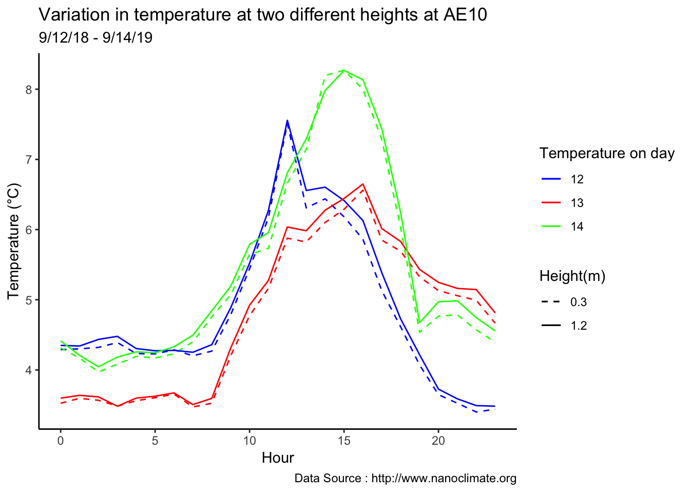
Microclim(Without the grid) - Take off title - Remove grid - Remove caption - Remove temperature on a day legend
decombined %>% filter(year(datec) %in% c(1981) & month(datec) %in% c(01) & day(datec) > 15 & day(datec) < 19) %>%
group_by(month,day,hr) %>%
ggplot() +
geom_line(aes(hr,Tsurface-273.5,group=day,color=as.factor(day),linetype = '0'),se=F)+ geom_line(aes(hr,TAH-273.5,group=day ,color=as.factor(day),linetype = '1.3'),se=F)+
scale_colour_manual("Temperature on day", breaks = c("16", "17","18"), values = c("blue","red","green"),guide = FALSE) +
scale_linetype_manual("Height(m)",values=c("0"=2,"1.3"=1)) +
theme_classic() + xlab("Hour") +
ylab("Temperature (°C)") + labs(colour = "Hour") 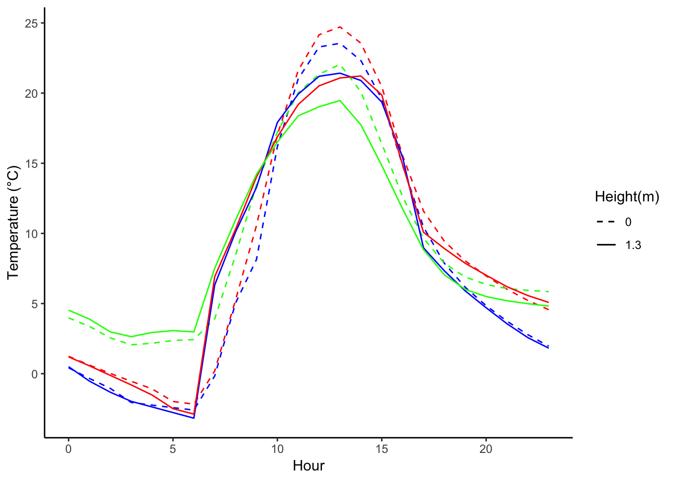 ## 12-02-2018
8.21 12-17-2018
Comparison to LaCrosse Weather Station
mclim_AE16_CN01_Calib<-read_csv('./data/AE16CN-Calbration.CSV')## Parsed with column specification:
## cols(
## date = col_character(),
## temp1 = col_double(),
## temp2 = col_double(),
## temp3 = col_double(),
## temp4 = col_double(),
## windspeed1 = col_double(),
## windspeed2 = col_double(),
## windspeed3 = col_double(),
## windspeed4 = col_double(),
## winddirection1 = col_double(),
## winddirection2 = col_double(),
## winddirection3 = col_double(),
## winddirection4 = col_double(),
## solar = col_double(),
## battery = col_double()
## )names(mclim_AE16_CN01_Calib)## [1] "date" "temp1" "temp2" "temp3"
## [5] "temp4" "windspeed1" "windspeed2" "windspeed3"
## [9] "windspeed4" "winddirection1" "winddirection2" "winddirection3"
## [13] "winddirection4" "solar" "battery"mclim_AE16_CN01_Calib$time <- as_datetime(mclim_AE16_CN01_Calib$date, format="%m/%d/%y %H:%M:%S",tz="America/Los_Angeles")
mclim_AE16_CN01_Calib$time <-as.POSIXct(mclim_AE16_CN01_Calib$time)
#Add hour month and day
## 11-05-2018
mclim_AE16_CN01_Calib$hr <- hour(mclim_AE16_CN01_Calib$time)
mclim_AE16_CN01_Calib$minute <- minute(mclim_AE16_CN01_Calib$time)
mclim_AE16_CN01_Calib$day <- day(mclim_AE16_CN01_Calib$time)
mclim_AE16_CN01_Calib$month<- month(mclim_AE16_CN01_Calib$time)Read in LaCrosse
library(weathermetrics)
LaCrosse_Calib<-read_csv('./data/LaCrosse_20181116-20181215.csv')
## Parsed with column specification:
## cols(
## Time = col_datetime(format = ""),
## HeatIndex_F = col_double(),
## `Humidity RH%` = col_double(),
## Temperature_F = col_double()
## )names(LaCrosse_Calib)## [1] "Time" "HeatIndex_F" "Humidity RH%" "Temperature_F"LaCrosse_Calib$Temperature_C<- weathermetrics::fahrenheit.to.celsius(LaCrosse_Calib$Temperature_F)
#LaCrosse_Calib$dtime <- as_datetime(LaCrosse_Calib$Time, format="%Y-%m-%d %H:%M:%S",tz="America/Los_Angeles")
#LaCrosse_Calib$dtime <-as.POSIXct(LaCrosse_Calib$Time)
#Add hour month and day
## 11-05-2018
LaCrosse_Calib$hr <- hour(LaCrosse_Calib$Time)
LaCrosse_Calib$minute <- minute(LaCrosse_Calib$Time)
LaCrosse_Calib$day <- day(LaCrosse_Calib$Time)
LaCrosse_Calib$month<- month(LaCrosse_Calib$Time)Raw plots
mclim_AE16_CN01_Calib %>% filter(day > 4) %>%
  ggplot() +
  geom_line(aes(time,temp1,col='A')) +
  geom_line(aes(time,temp2,col='B')) +
  geom_line(data=LaCrosse_Calib, aes(Time,Temperature_C,col='C')) +

   theme_classic() + labs(x="Date", y="Temperature(°C) ",subtitle="Microclimate station -  AE10 Validation ",                                                                                                   caption="Data Source : http://nanoclimate.org") +
   geom_hline(aes(yintercept=9),colour="black", linetype="dashed")  +
    scale_colour_manual(name = 'Heights',
         values =c('A'='red','B'='blue','C'='green'), labels = c('1.2','.9',"Reference"))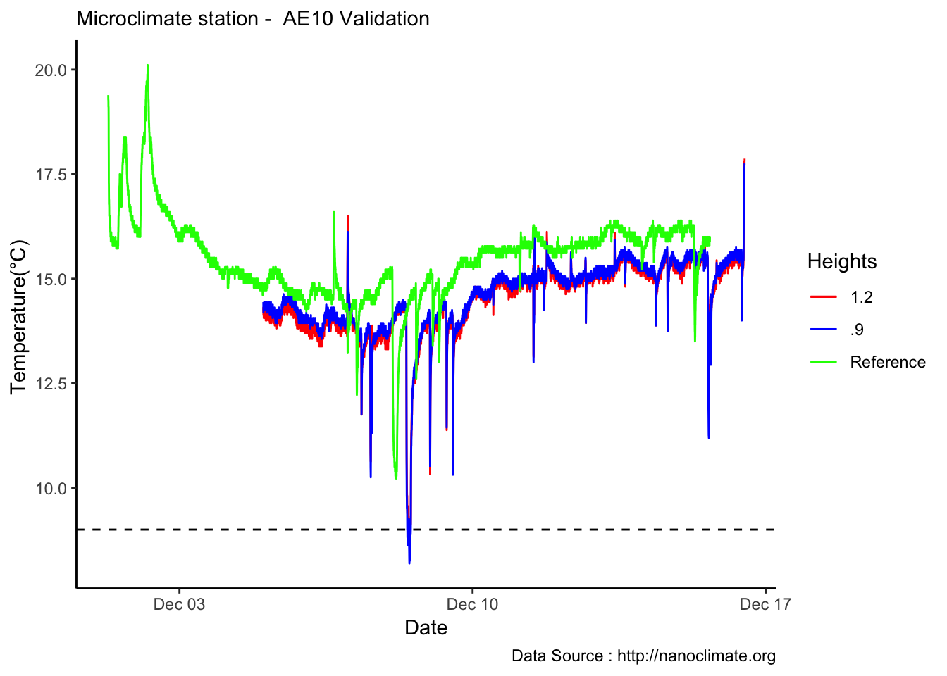
Hourly
8.22 12-21-2018
Plot three elevations at Mt Rainier
MtRainier_Local <- read_csv('./data/mt-rainier_temperature_2018.csv')## Parsed with column specification:
## cols(
## `Date/Time (PST)` = col_datetime(format = ""),
## `deg F - 5400' - Paradise` = col_double(),
## `deg F - 6410' - Sunrise Base` = col_double(),
## `deg F - 6880' - Sunrise Upper` = col_double(),
## `deg F - 10110' - Camp Muir` = col_double()
## )colnames(MtRainier_Local) <- c('datetime','Paradise_5400','Sunrise_6410','Sunrise_6880','CampMuir_10110')
MtRainier_Local$hr <- hour(MtRainier_Local$datetime)
MtRainier_Local$minute <- minute(MtRainier_Local$datetime)
MtRainier_Local$day <- day(MtRainier_Local$datetime)
MtRainier_Local$month<- month(MtRainier_Local$datetime)
MtRainier_Local$year<- year(MtRainier_Local$datetime)
MtRainier_Local %>% filter(month == 9 & year== 2018 ) %>%
ggplot() +
geom_line(aes(datetime,weathermetrics::fahrenheit.to.celsius(Paradise_5400),col='5400')) +
geom_line(aes(datetime,weathermetrics::fahrenheit.to.celsius(Sunrise_6410),col='6410')) +
geom_line(aes(datetime,weathermetrics::fahrenheit.to.celsius(Sunrise_6880),col='6880')) +
theme_classic() + labs(x="Date", y="Temperature(°C) ",subtitle="Microclimate station - AE10 Validation ", caption="Data Source : http://nanoclimate.org") +
geom_hline(aes(yintercept=9),colour="black", linetype="dashed") +
scale_colour_manual(name = 'Heights',
values =c('5400'='red','6410'='blue','6880'='green'), labels = c('5400','6410',"6880"))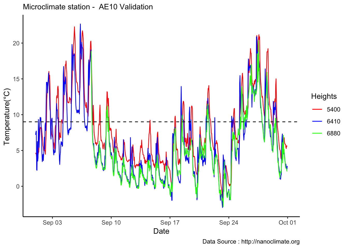
Read and plot the points
#With zero plane dispacement
library(leaflet)

Nodes <- read_csv('./data/Nodes-Table 1.csv')
## Parsed with column specification:
## cols(
## X1 = col_logical(),
## NodeId = col_character(),
## Lat = col_double(),
## Long = col_double(),
## Type = col_character(),
## Canopy = col_character(),
## `Live Date(GMT)` = col_character(),
## Notes = col_character()
## )Nodes %>% leaflet() %>%
fitBounds(~min(Long), ~min(Lat), ~max(Long), ~max(Lat)) %>%
addProviderTiles(providers$Esri.WorldTopoMap,
options = providerTileOptions(noWrap = TRUE)
) %>%
addMarkers(~Long,~Lat,popup = ~as.character(NodeId), label = ~as.character(NodeId)) %>%
addCircleMarkers(-121.73,46.79,color = "red") #addCircles(~lon,~lat,color = ~pal(estElevation)) %>%
#addLegend(pal = pal, values = ~estElevation)
## Get long and lat from your data.frame. Make sure that the order is in lon/lat.
xy <- Nodes[,c('Long','Lat')]
spdf <- SpatialPointsDataFrame(coords = xy, data = Nodes,
proj4string = CRS("+proj=longlat +datum=WGS84 +ellps=WGS84 +towgs84=0,0,0"))
prj_dd <- "+proj=longlat +ellps=WGS84 +datum=WGS84 +no_defs"
library(elevatr)
df_elev_epqs <- get_elev_point(spdf, prj = prj_dd, src = "epqs")## Note: Elevation units are in &units=Meters
## Note:. The coordinate reference system is:
## +proj=longlat +datum=WGS84 +ellps=WGS84 +towgs84=0,0,0Plot the nodes on high resolution DEM
#With zero plane dispacement
library(rgdal) #this package is necessary to import the .asc file in R.
library(rasterVis) #this package has the function which allows the 3D plotting.

#set the path where the file is, and import it into R.
r= raster(paste("./data/rainier_2007_dtm_12.tif", sep=""))

#visualize the raster in 3D
plot(r,lit=TRUE)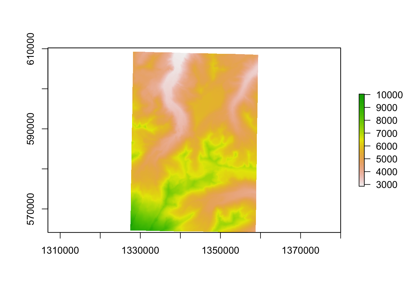
8.23 1-3-2019
Checking a sample day at Mt Rainier, testing the hypothesis that temperature decreases by elevation. We are going to look at sample day of September 12th 2018, we see for for couple of hours temperature shows inversion. Now, unstable of the boundary layer means mixing, usually results from the wind.
MtRainier_Local <- read_csv('./data/mt-rainier_temperature_2018.csv')## Parsed with column specification:
## cols(
## `Date/Time (PST)` = col_datetime(format = ""),
## `deg F - 5400' - Paradise` = col_double(),
## `deg F - 6410' - Sunrise Base` = col_double(),
## `deg F - 6880' - Sunrise Upper` = col_double(),
## `deg F - 10110' - Camp Muir` = col_double()
## )colnames(MtRainier_Local) <- c('datetime','Paradise_5400','Sunrise_6410','Sunrise_6880','CampMuir_10110')
MtRainier_Local$hr <- hour(MtRainier_Local$datetime)
MtRainier_Local$minute <- minute(MtRainier_Local$datetime)
MtRainier_Local$day <- day(MtRainier_Local$datetime)
MtRainier_Local$month<- month(MtRainier_Local$datetime)
MtRainier_Local$year<- year(MtRainier_Local$datetime)
MtRainier_Local %>% filter(month == 9 & year== 2018 & day == 12) %>%
ggplot() +
geom_line(aes(datetime,weathermetrics::fahrenheit.to.celsius(Paradise_5400),col='1645')) +
geom_line(aes(datetime,weathermetrics::fahrenheit.to.celsius(Sunrise_6410),col='1953')) +
geom_line(aes(datetime,weathermetrics::fahrenheit.to.celsius(Sunrise_6880),col='2097')) +
geom_line(aes(datetime,weathermetrics::fahrenheit.to.celsius(CampMuir_10110),col='3081')) +
theme_classic() + labs(x="Date", y="Temperature(°C) ",subtitle="Met stations - Mt Rainier ", caption="Data Source : http://nanoclimate.org") +
scale_colour_manual(name = 'Heights(m)',
values =c('1','2','3','4'), labels = c('1645','1953',"2097","3081")) +
geom_hline(aes(yintercept=9),colour="black", linetype="dashed") 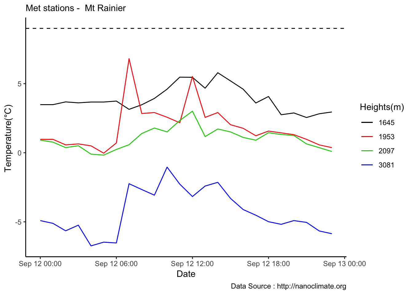
Lets lookjust for September
MtRainier_Local <- read_csv('./data/mt-rainier_temperature_2018.csv')## Parsed with column specification:
## cols(
## `Date/Time (PST)` = col_datetime(format = ""),
## `deg F - 5400' - Paradise` = col_double(),
## `deg F - 6410' - Sunrise Base` = col_double(),
## `deg F - 6880' - Sunrise Upper` = col_double(),
## `deg F - 10110' - Camp Muir` = col_double()
## )colnames(MtRainier_Local) <- c('datetime','Paradise_5400','Sunrise_6410','Sunrise_6880','CampMuir_10110')
MtRainier_Local$hr <- hour(MtRainier_Local$datetime)
MtRainier_Local$minute <- minute(MtRainier_Local$datetime)
MtRainier_Local$day <- day(MtRainier_Local$datetime)
MtRainier_Local$month<- month(MtRainier_Local$datetime)
MtRainier_Local$year<- year(MtRainier_Local$datetime)
MtRainier_Local %>% filter(month == 9 & year== 2018 ) %>%
ggplot() +
geom_line(aes(datetime,weathermetrics::fahrenheit.to.celsius(Paradise_5400),col='1645')) +
geom_line(aes(datetime,weathermetrics::fahrenheit.to.celsius(Sunrise_6410),col='1953')) +
geom_line(aes(datetime,weathermetrics::fahrenheit.to.celsius(Sunrise_6880),col='2097')) +
geom_line(aes(datetime,weathermetrics::fahrenheit.to.celsius(CampMuir_10110),col='3081')) +
theme_classic() + labs(x="Date", y="Temperature(°C) ",subtitle="Met stations - Mt Rainier Hourly readings (2018) ", caption="Data Source : http://nwac.us") +
scale_colour_manual(name = 'Heights(m)',
values =c('1','2','3','4'), labels = c('1645','1953',"2097","3081")) +
geom_hline(aes(yintercept=9),colour="black", linetype="dashed") 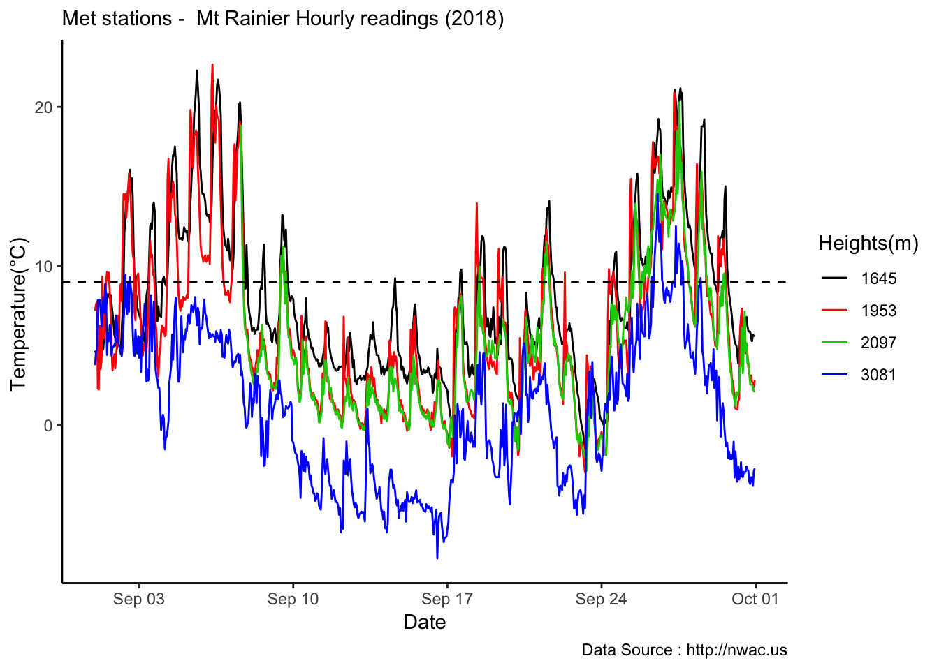
See if it is true for the whole year,looks like Summer is bit jumbled
MtRainier_Local <- read_csv('./data/mt-rainier_temperature_2018.csv')## Parsed with column specification:
## cols(
## `Date/Time (PST)` = col_datetime(format = ""),
## `deg F - 5400' - Paradise` = col_double(),
## `deg F - 6410' - Sunrise Base` = col_double(),
## `deg F - 6880' - Sunrise Upper` = col_double(),
## `deg F - 10110' - Camp Muir` = col_double()
## )colnames(MtRainier_Local) <- c('datetime','Paradise_5400','Sunrise_6410','Sunrise_6880','CampMuir_10110')
MtRainier_Local$hr <- hour(MtRainier_Local$datetime)
MtRainier_Local$minute <- minute(MtRainier_Local$datetime)
MtRainier_Local$day <- day(MtRainier_Local$datetime)
MtRainier_Local$month<- month(MtRainier_Local$datetime)
MtRainier_Local$year<- year(MtRainier_Local$datetime)
MtRainier_Local %>% filter( year== 2018) %>%
ggplot() +
geom_smooth(method = "loess",aes(datetime,weathermetrics::fahrenheit.to.celsius(Paradise_5400),colour='1645'),se=TRUE) +
geom_smooth(method = "loess",aes(datetime,weathermetrics::fahrenheit.to.celsius(Sunrise_6410),colour='1953'),se=TRUE) +
geom_smooth(method = "loess",aes(datetime,weathermetrics::fahrenheit.to.celsius(Sunrise_6880),colour='2097'),se=TRUE) +
geom_smooth(method = "loess",aes(datetime,weathermetrics::fahrenheit.to.celsius(CampMuir_10110),colour='3081'),se=TRUE) +
theme_classic() + labs(x="Date", y="Temperature(°C) ",subtitle="Met stations - Mt Rainier ", caption="Data Source : http://nwac.us") +
scale_colour_manual(name = 'Heights(m)',
values =c('1','2','3','4'), labels = c('1645','1953',"2097","3081")) +
geom_hline(aes(yintercept=9),colour="black", linetype="dashed") 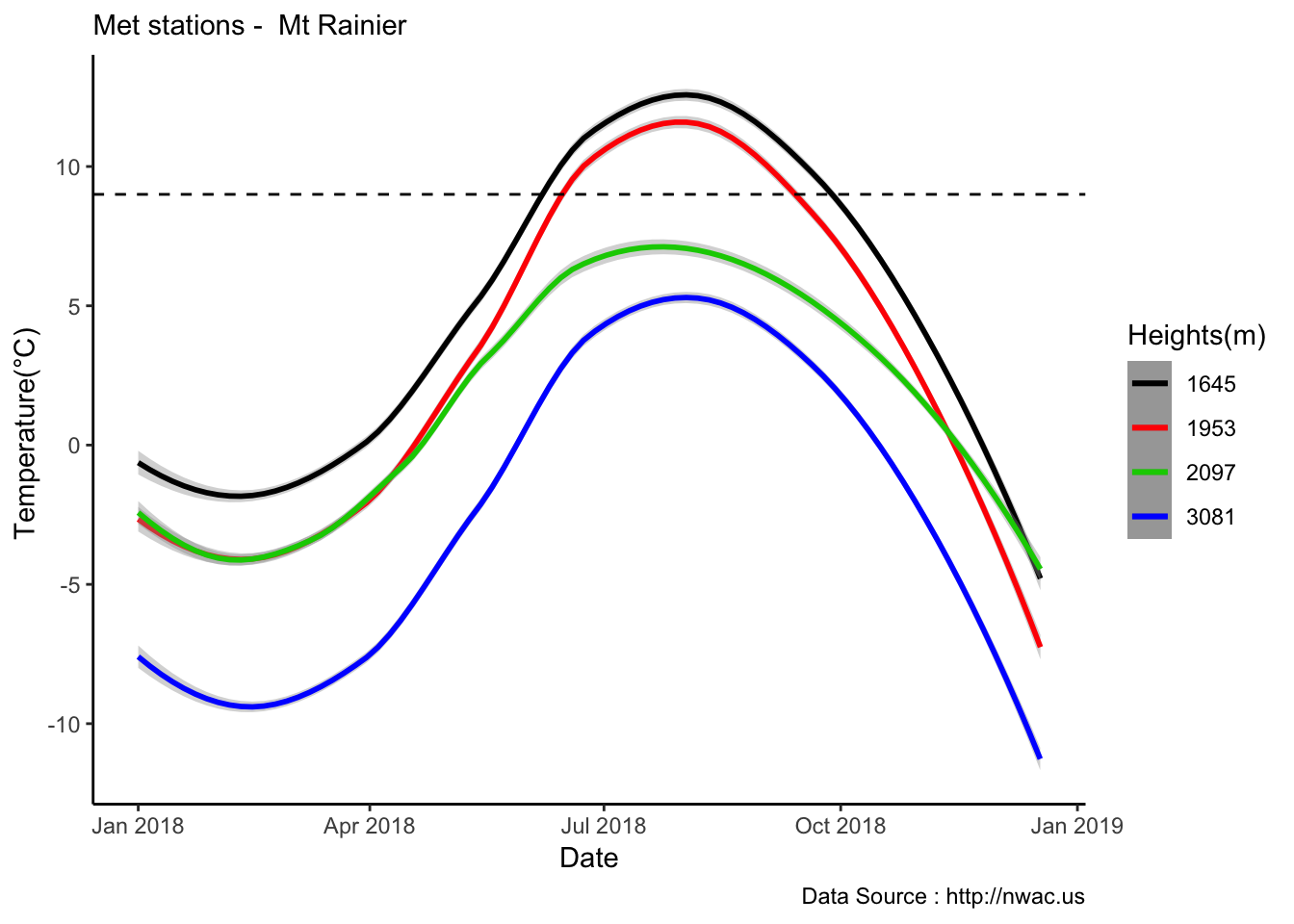 Mapping solar radiation for the same three heights.Its generally truethat higher the elevation,more solar insolation,but must not bethe case in all as
MtRainier_Solar <- read_csv('./data/mt-rainier_solar_pyranometer_2018.csv')## Parsed with column specification:
## cols(
## `Date/Time (PST)` = col_datetime(format = ""),
## `W/m2 - 5380' - Paradise Wind` = col_double(),
## `W/m2 - 6880' - Sunrise Upper` = col_double(),
## `W/m2 - 10110' - Camp Muir` = col_double()
## )colnames(MtRainier_Solar) <- c('datetime','Paradise_5400','Sunrise_6880','CampMuir_10110')
MtRainier_Solar$hr <- hour(MtRainier_Solar$datetime)
MtRainier_Solar$minute <- minute(MtRainier_Solar$datetime)
MtRainier_Solar$day <- day(MtRainier_Solar$datetime)
MtRainier_Solar$month<- month(MtRainier_Solar$datetime)
MtRainier_Solar$year<- year(MtRainier_Solar$datetime)
MtRainier_Solar %>% filter(month == 9 & year== 2018 & day == 10) %>%
ggplot() +
geom_line(aes(datetime,Paradise_5400,col='1645')) +
geom_line(aes(datetime,Sunrise_6880,col='2097')) +
geom_line(aes(datetime,CampMuir_10110,col='3081')) +
theme_classic() + labs(x="Date", y="Solar radiation(W/m2) ",subtitle="Met stations - Mt Rainier Solar ", caption="Data Source : http://nanoclimate.org") +
geom_hline(aes(yintercept=9),colour="black", linetype="dashed") +
scale_colour_manual(name = 'Heights(m)',
values =c('red','blue','green'), labels = c('1645','2097',"3081"))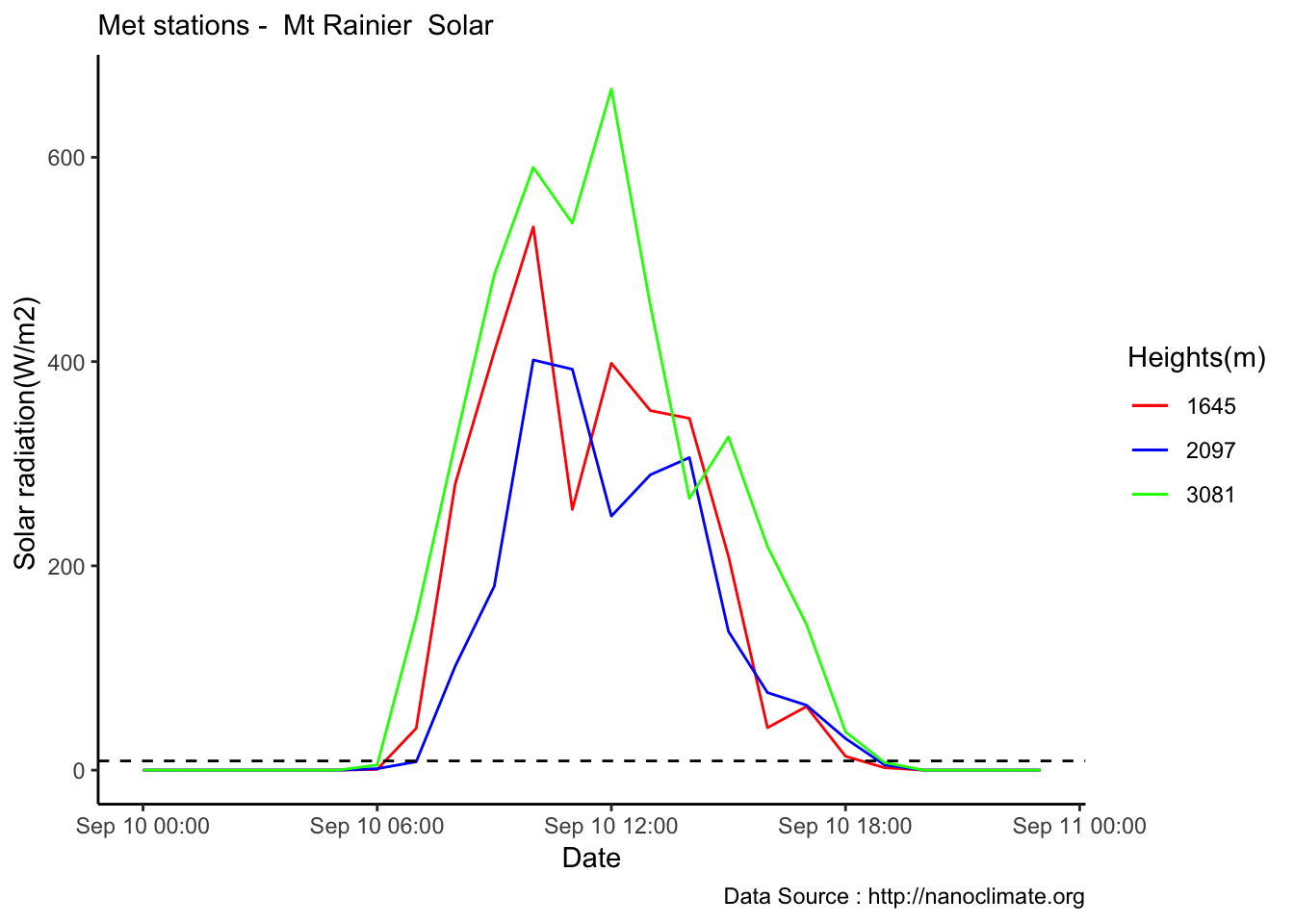
Lets look for whole of September
MtRainier_Solar <- read_csv('./data/mt-rainier_solar_pyranometer_2018.csv')## Parsed with column specification:
## cols(
## `Date/Time (PST)` = col_datetime(format = ""),
## `W/m2 - 5380' - Paradise Wind` = col_double(),
## `W/m2 - 6880' - Sunrise Upper` = col_double(),
## `W/m2 - 10110' - Camp Muir` = col_double()
## )colnames(MtRainier_Solar) <- c('datetime','Paradise_5400','Sunrise_6880','CampMuir_10110')
MtRainier_Solar$hr <- hour(MtRainier_Solar$datetime)
MtRainier_Solar$minute <- minute(MtRainier_Solar$datetime)
MtRainier_Solar$day <- day(MtRainier_Solar$datetime)
MtRainier_Solar$month<- month(MtRainier_Solar$datetime)
MtRainier_Solar$year<- year(MtRainier_Solar$datetime)
MtRainier_Solar %>% filter(month == 9 & year== 2018 ) %>%
ggplot() +
geom_line(aes(datetime,Paradise_5400,col='1645')) +
geom_line(aes(datetime,Sunrise_6880,col='2097')) +
geom_line(aes(datetime,CampMuir_10110,col='3081')) +
theme_classic() + labs(x="Date", y="Solar radiation(W/m2) ",subtitle="Met stations - Mt Rainier Solar ", caption="Data Source : http://nanoclimate.org") +
geom_hline(aes(yintercept=9),colour="black", linetype="dashed") +
scale_colour_manual(name = 'Heights(m)',
values =c('red','blue','green'), labels = c('1645','2097',"3081"))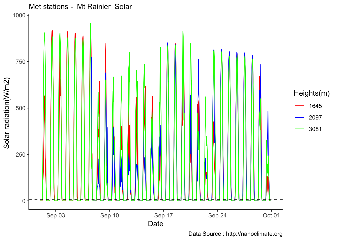
Highest elevation crowding,lets take it out
MtRainier_Solar <- read_csv('./data/mt-rainier_solar_pyranometer_2018.csv')## Parsed with column specification:
## cols(
## `Date/Time (PST)` = col_datetime(format = ""),
## `W/m2 - 5380' - Paradise Wind` = col_double(),
## `W/m2 - 6880' - Sunrise Upper` = col_double(),
## `W/m2 - 10110' - Camp Muir` = col_double()
## )colnames(MtRainier_Solar) <- c('datetime','Paradise_5400','Sunrise_6880','CampMuir_10110')
MtRainier_Solar$hr <- hour(MtRainier_Solar$datetime)
MtRainier_Solar$minute <- minute(MtRainier_Solar$datetime)
MtRainier_Solar$day <- day(MtRainier_Solar$datetime)
MtRainier_Solar$month<- month(MtRainier_Solar$datetime)
MtRainier_Solar$year<- year(MtRainier_Solar$datetime)
MtRainier_Solar %>% filter(month == 9 & year== 2018 ) %>%
ggplot() +
geom_line(aes(datetime,Paradise_5400,col='1645')) +
geom_line(aes(datetime,Sunrise_6880,col='2097')) +
theme_classic() + labs(x="Date", y="Solar radiation(W/m2) ",subtitle="Met stations - Mt Rainier Solar ", caption="Data Source : http://nanoclimate.org") +
geom_hline(aes(yintercept=9),colour="black", linetype="dashed") +
scale_colour_manual(name = 'Heights(m)',
values =c('red','blue','green'), labels = c('1645','2097',"3081"))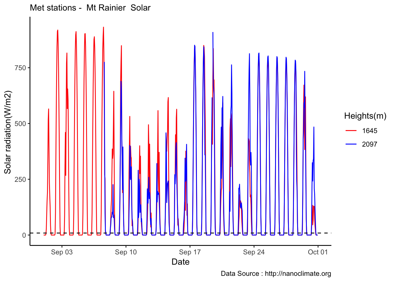
Day in, selective days, again the solar insolation although highest at higher elevastions, not really a function of elevation
MtRainier_Solar <- read_csv('./data/mt-rainier_solar_pyranometer_2018.csv')## Parsed with column specification:
## cols(
## `Date/Time (PST)` = col_datetime(format = ""),
## `W/m2 - 5380' - Paradise Wind` = col_double(),
## `W/m2 - 6880' - Sunrise Upper` = col_double(),
## `W/m2 - 10110' - Camp Muir` = col_double()
## )colnames(MtRainier_Solar) <- c('datetime','Paradise_5400','Sunrise_6880','CampMuir_10110')
MtRainier_Solar$hr <- hour(MtRainier_Solar$datetime)
MtRainier_Solar$minute <- minute(MtRainier_Solar$datetime)
MtRainier_Solar$day <- day(MtRainier_Solar$datetime)
MtRainier_Solar$month<- month(MtRainier_Solar$datetime)
MtRainier_Solar$year<- year(MtRainier_Solar$datetime)
MtRainier_Solar %>% filter(month == 9 & year== 2018 & day %in% c(10,11,12,13,14) ) %>%
ggplot() +
geom_line(aes(datetime,Paradise_5400,col='1645')) +
geom_line(aes(datetime,Sunrise_6880,col='2097')) +
geom_line(aes(datetime,CampMuir_10110,col='3081')) +
theme_classic() + labs(x="Date", y="Solar radiation(W/m2) ",subtitle="Met stations - Mt Rainier Solar - 2018", caption="Data Source : http://nanoclimate.org") +
geom_hline(aes(yintercept=9),colour="black", linetype="dashed") +
scale_colour_manual(name = 'Heights(m)',
values =c('red','blue','green'), labels = c('1645','2097',"3081"))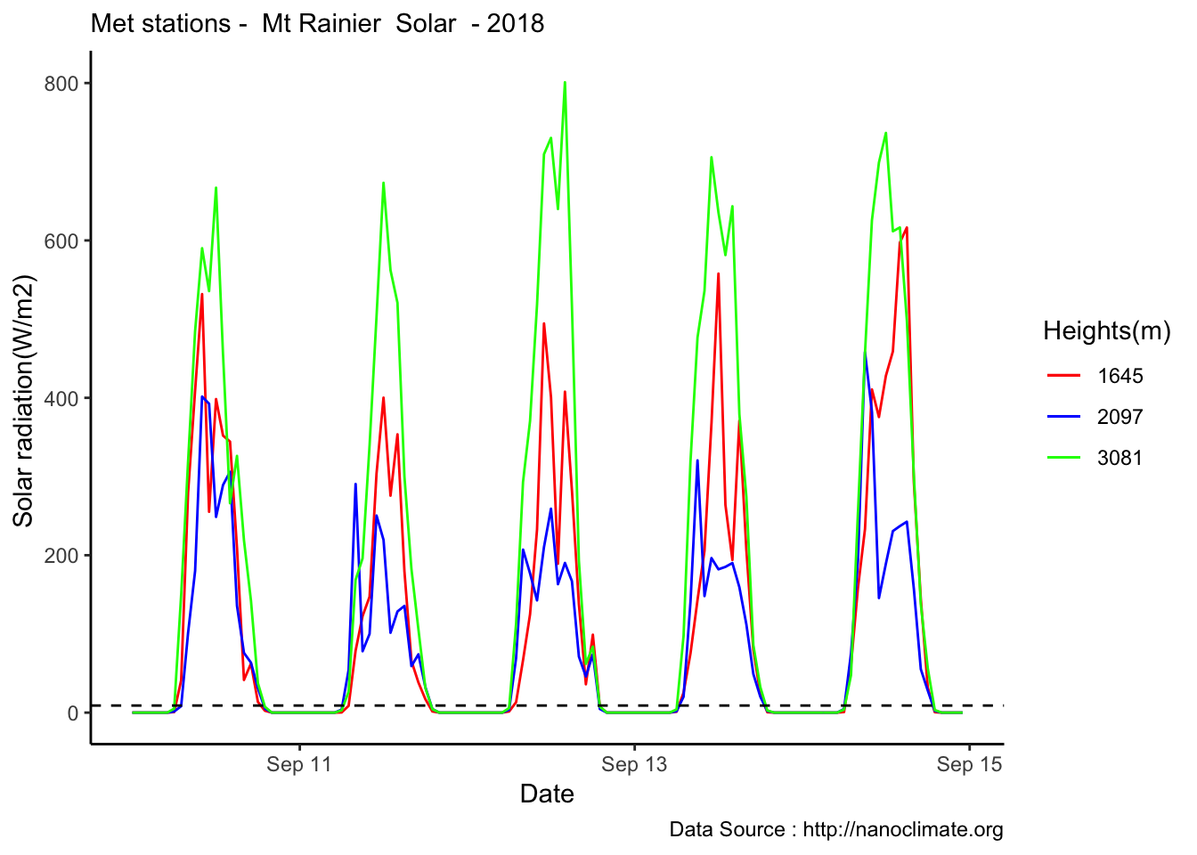 Lets read in A1 temps , plotting only September 2016
MtRainier_AE10A1_1617 <- read_csv('./data/AE10-A1-061616-062717.csv')## Parsed with column specification:
## cols(
## `#` = col_double(),
## `Date Time, GMT-07:00` = col_character(),
## `Temp, °C (LGR S/N: 10620921, SEN S/N: 10620921)` = col_double(),
## `Coupler Attached (LGR S/N: 10620921)` = col_logical(),
## `Host Connected (LGR S/N: 10620921)` = col_logical(),
## `Coupler Detached (LGR S/N: 10620921)` = col_logical(),
## `Stopped (LGR S/N: 10620921)` = col_logical(),
## `End Of File (LGR S/N: 10620921)` = col_logical()
## )colnames(MtRainier_AE10A1_1617) <- c('#','datetime','Temp','CoupAttach','HostConn','CoupDeAttach','Stopped','eof')
MtRainier_AE10A1_1617$timect <- as.POSIXct(MtRainier_AE10A1_1617$datetime, format="%m/%d/%y %I:%M:%S %p",tz="America/Los_Angeles")
MtRainier_AE10A1_1617$hr <- hour(MtRainier_AE10A1_1617$timect)
MtRainier_AE10A1_1617$minute <- minute(MtRainier_AE10A1_1617$timect)
MtRainier_AE10A1_1617$day <- day(MtRainier_AE10A1_1617$timect)
MtRainier_AE10A1_1617$month<- month(MtRainier_AE10A1_1617$timect)
MtRainier_AE10A1_1617$year<- year(MtRainier_AE10A1_1617$timect)
MtRainier_AE10A1_1617 %>%
filter(month == 9 & year== 2016 & day %in% c(10,11,12,13,14) ) %>%
ggplot() +
geom_point(aes(timect,Temp,col='A1')) +
geom_line(aes(timect,Temp)) +
theme_classic() + labs(x="Date", y="Temperature(°C) ",subtitle="Air hobo AE10 A1 - Mt Rainie -Recorded every 2 hours (2016) ", caption="Data Source : JHRL") +
geom_hline(aes(yintercept=9),colour="black", linetype="dashed") +
scale_colour_manual(name = 'Heights(m)',
values =c('red','blue','green'), labels = c('1645','2097',"3081"))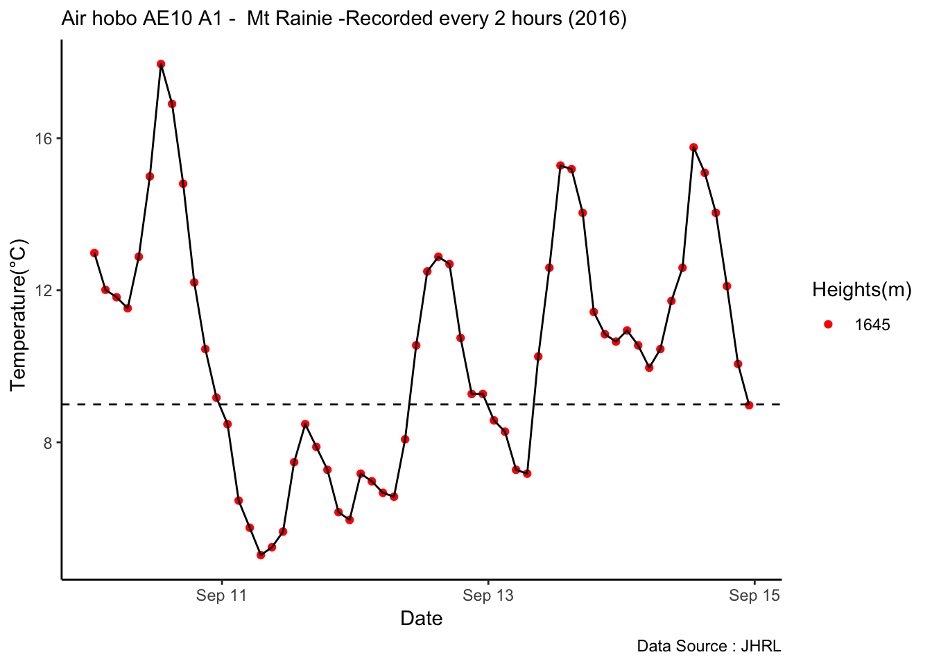
Lets read in A1 temps , plotting only September 2017
MtRainier_AE10A1_1718 <- read_csv('./data/AE10-A1-062817-072818.csv')## Parsed with column specification:
## cols(
## `#` = col_double(),
## `Date Time, GMT-07:00` = col_character(),
## `Temp, °C (LGR S/N: 10620922, SEN S/N: 10620922)` = col_double(),
## `Coupler Attached (LGR S/N: 10620922)` = col_logical(),
## `Host Connected (LGR S/N: 10620922)` = col_logical(),
## `Stopped (LGR S/N: 10620922)` = col_logical(),
## `End Of File (LGR S/N: 10620922)` = col_logical()
## )colnames(MtRainier_AE10A1_1718) <- c('#','datetime','Temp','CoupAttach','HostConn','Stopped','eof')
MtRainier_AE10A1_1718$timect <- as.POSIXct(MtRainier_AE10A1_1718$datetime, format="%m/%d/%y %I:%M:%S %p",tz="America/Los_Angeles")
#MtRainier_AE10A1_1718$timect <- as.POSIXct(MtRainier_AE10A1_1718$datetime, format="%m/%d/%y %I:%M:%S %p",tz="America/Los_Angeles")
MtRainier_AE10A1_1718$hr <- hour(MtRainier_AE10A1_1718$timect)
MtRainier_AE10A1_1718$minute <- minute(MtRainier_AE10A1_1718$timect)
MtRainier_AE10A1_1718$day <- day(MtRainier_AE10A1_1718$timect)
MtRainier_AE10A1_1718$month<- month(MtRainier_AE10A1_1718$timect)
MtRainier_AE10A1_1718$year<- year(MtRainier_AE10A1_1718$timect)
MtRainier_AE10A1_1718 %>%
filter(month == 9 & year== 2017 & day %in% c(10,11,12,13,14) ) %>%
ggplot() +
geom_point(aes(timect,Temp,col='A1')) +
geom_line(aes(timect,Temp)) +
theme_classic() + labs(x="Date", y="Temperature(°C) ",subtitle="Air hobo AE10 A1 - Mt Rainie -Recorded every 2 hours (2017) ", caption="Data Source : JHRL") +
geom_hline(aes(yintercept=9),colour="black", linetype="dashed") +
scale_colour_manual(name = 'Heights(m)',
values =c('red','blue','green'), labels = c('1645','2097',"3081"))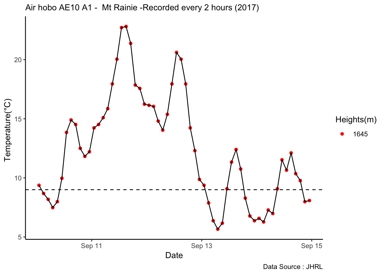
How does Sept compare to Paradise (2017)
# read in Paradise

MtRainier_Local_2017<- read_csv('./data/mt-rainier_temperature_2017.csv')
## Parsed with column specification:
## cols(
## `Date/Time (PST)` = col_datetime(format = ""),
## `deg F - 5400' - Paradise` = col_double(),
## `deg F - 6410' - Sunrise Base` = col_double(),
## `deg F - 6880' - Sunrise Upper` = col_double(),
## `deg F - 10110' - Camp Muir` = col_double()
## )colnames(MtRainier_Local_2017) <- c('datetime','Paradise_5400','Sunrise_6410','Sunrise_6880','CampMuir_10110')
MtRainier_Local_2017$hr <- hour(MtRainier_Local_2017$datetime)
MtRainier_Local_2017$minute <- minute(MtRainier_Local_2017$datetime)
MtRainier_Local_2017$day <- day(MtRainier_Local_2017$datetime)
MtRainier_Local_2017$month<- month(MtRainier_Local_2017$datetime)
MtRainier_Local_2017$year<- year(MtRainier_Local_2017$datetime)
MtRainier_Local_2017 %>% filter(month == 9 & year== 2017 ) %>%
ggplot() +
geom_line(aes(datetime,weathermetrics::fahrenheit.to.celsius(Paradise_5400),col='1645')) +
geom_line(aes(datetime,weathermetrics::fahrenheit.to.celsius(Sunrise_6410),col='1953')) +
geom_line(aes(datetime,weathermetrics::fahrenheit.to.celsius(Sunrise_6880),col='2097')) +
geom_line(aes(datetime,weathermetrics::fahrenheit.to.celsius(CampMuir_10110),col='3081')) +
theme_classic() + labs(x="Date", y="Temperature(°C) ",subtitle="Met stations - Mt Rainier Hourly readings (2017) ", caption="Data Source : http://nwac.us") +
scale_colour_manual(name = 'Heights(m)',
values =c('1','2','3','4'), labels = c('1645','1953',"2097","3081")) +
geom_hline(aes(yintercept=9),colour="black", linetype="dashed") 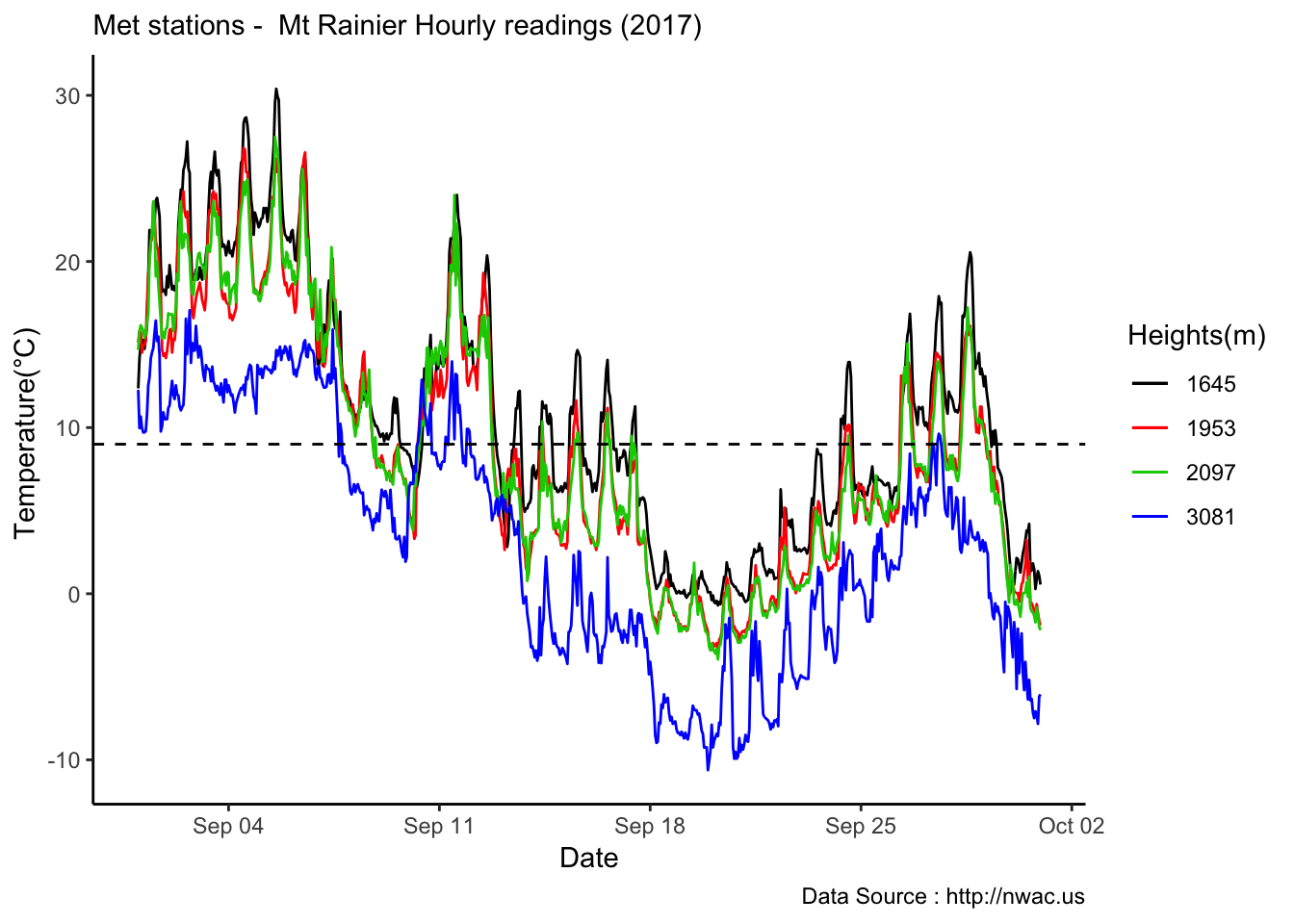
MtRainier_AE10A1_1718 <- read_csv('./data/AE10-A1-062817-072818.csv')## Parsed with column specification:
## cols(
## `#` = col_double(),
## `Date Time, GMT-07:00` = col_character(),
## `Temp, °C (LGR S/N: 10620922, SEN S/N: 10620922)` = col_double(),
## `Coupler Attached (LGR S/N: 10620922)` = col_logical(),
## `Host Connected (LGR S/N: 10620922)` = col_logical(),
## `Stopped (LGR S/N: 10620922)` = col_logical(),
## `End Of File (LGR S/N: 10620922)` = col_logical()
## )colnames(MtRainier_AE10A1_1718) <- c('#','datetime','Temp','CoupAttach','HostConn','Stopped','eof')
MtRainier_AE10A1_1718$timect <- as.POSIXct(MtRainier_AE10A1_1718$datetime, format="%m/%d/%y %I:%M:%S %p",tz="America/Los_Angeles")
MtRainier_AE10A1_1718$hr <- hour(MtRainier_AE10A1_1718$timect)
MtRainier_AE10A1_1718$minute <- minute(MtRainier_AE10A1_1718$timect)
MtRainier_AE10A1_1718$day <- day(MtRainier_AE10A1_1718$timect)
MtRainier_AE10A1_1718$month<- month(MtRainier_AE10A1_1718$timect)
MtRainier_AE10A1_1718$year<- year(MtRainier_AE10A1_1718$timect)
MtRainier_AE10A1_1718 %>%
filter(month == 9 & year== 2017 ) %>%
ggplot() +
geom_point(aes(timect,Temp,col='A1')) +
geom_line(aes(timect,Temp)) +
theme_classic() + labs(x="Date", y="Temperature(°C) ",subtitle="Air hobo AE10 A1 - Mt Rainie -Recorded every 2 hours (2017) ", caption="Data Source : JHRL") +
geom_hline(aes(yintercept=9),colour="black", linetype="dashed") +
scale_colour_manual(name = 'Heights(m)',
values =c('red','blue','green'), labels = c('1645','2097',"3081"))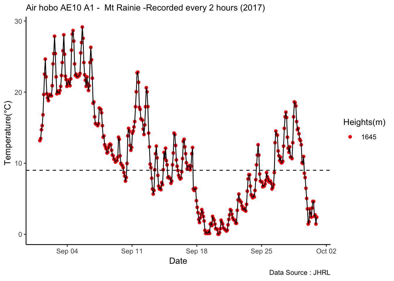
Combine whole month with A1
# read in Paradise

MtRainier_Local_2017 %>% filter(month == 9 & year== 2017 ) %>%
  ggplot() +
  geom_line(aes(datetime,weathermetrics::fahrenheit.to.celsius(Paradise_5400),col='1645')) +
  geom_line(aes(datetime,weathermetrics::fahrenheit.to.celsius(Sunrise_6410),col='1953')) +
  geom_line(aes(datetime,weathermetrics::fahrenheit.to.celsius(Sunrise_6880),col='2097')) +
  geom_line(aes(datetime,weathermetrics::fahrenheit.to.celsius(CampMuir_10110),col='3081')) +
  geom_line(data=MtRainier_AE10A1_1718[MtRainier_AE10A1_1718$month == 9 & MtRainier_AE10A1_1718$year== 2017,],aes(timect,Temp,col='1450')) +
theme_classic() + labs(x="Date", y="Temperature(°C) ", color = "Height (m)",
                       subtitle="Met stations and A1-  Mt Rainier Hourly readings (2017) ",                                                                                                   caption="Data Source : http://nwac.us")  +
geom_hline(aes(yintercept=9),colour="black", linetype="dashed") 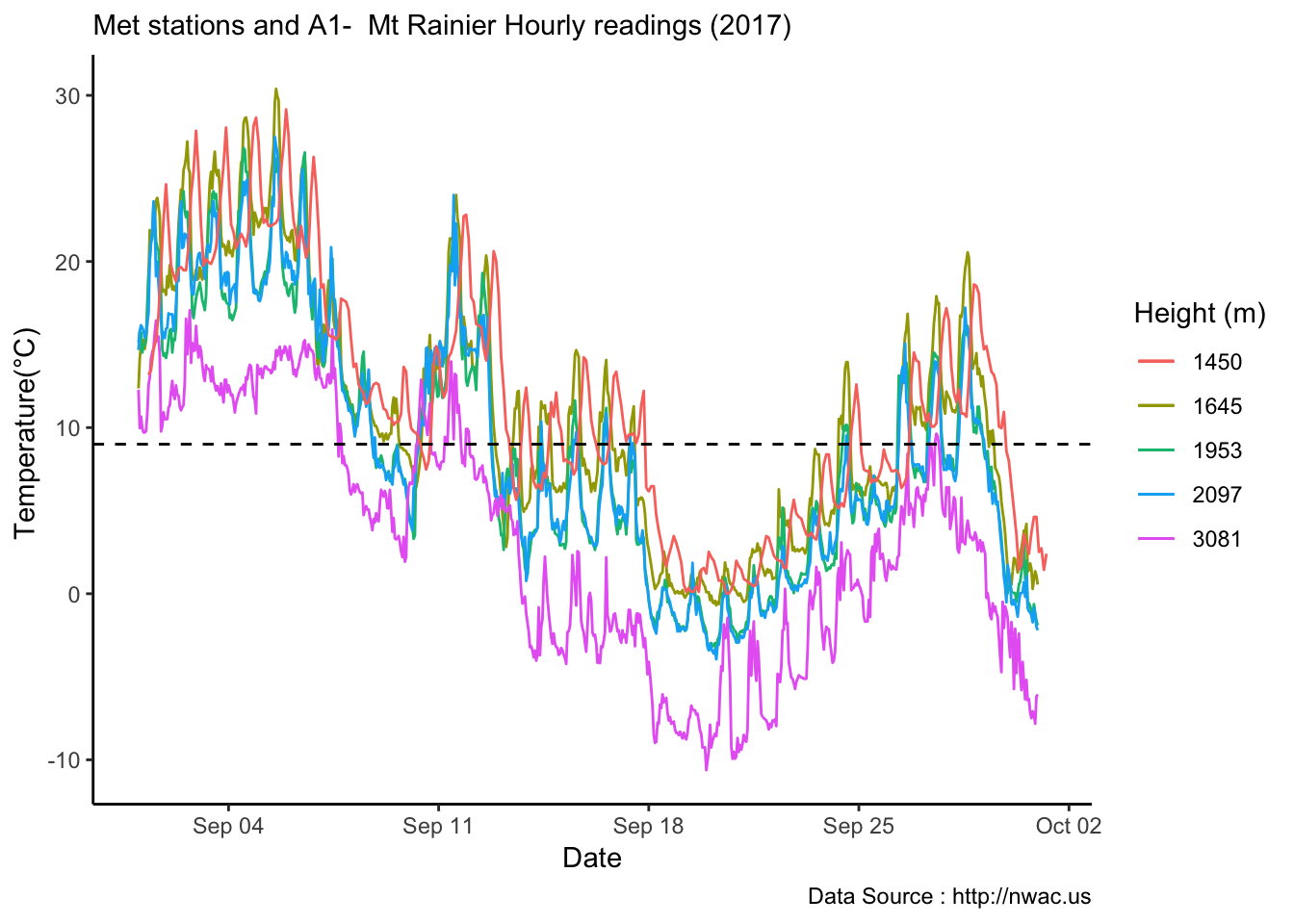
Combine whole month with A1 selective days
# read in Paradise
MtRainier_AE10A1_1718$timectdiff2 <- MtRainier_AE10A1_1718$timect - lubridate::hours(2)

MtRainier_Local_2017 %>% filter(month == 9 & year== 2017 & day %in% c(1,2,3,4,5,10,11,12,13,14,15) ) %>%
  ggplot() +
  geom_line(aes(datetime,weathermetrics::fahrenheit.to.celsius(Paradise_5400),col='1645')) +
  geom_line(aes(datetime,weathermetrics::fahrenheit.to.celsius(Sunrise_6410),col='1953')) +
  geom_line(aes(datetime,weathermetrics::fahrenheit.to.celsius(Sunrise_6880),col='2097')) +
  geom_line(aes(datetime,weathermetrics::fahrenheit.to.celsius(CampMuir_10110),col='3081')) +
  geom_line(data=MtRainier_AE10A1_1718[MtRainier_AE10A1_1718$month == 9 &      MtRainier_AE10A1_1718$year== 2017 & MtRainier_AE10A1_1718$day %in% c(1,2,3,4,5,10,11,12,13,14,15) ,],aes(timectdiff2,Temp,col='1450')) +
theme_classic() + labs(x="Date", y="Temperature(°C) ", color = "Height (m)",
                       subtitle="Met stations and A1-  Mt Rainier Hourly readings (2017) ",                                                                                                   caption="Data Source : http://nwac.us")  +
geom_hline(aes(yintercept=9),colour="black", linetype="dashed") 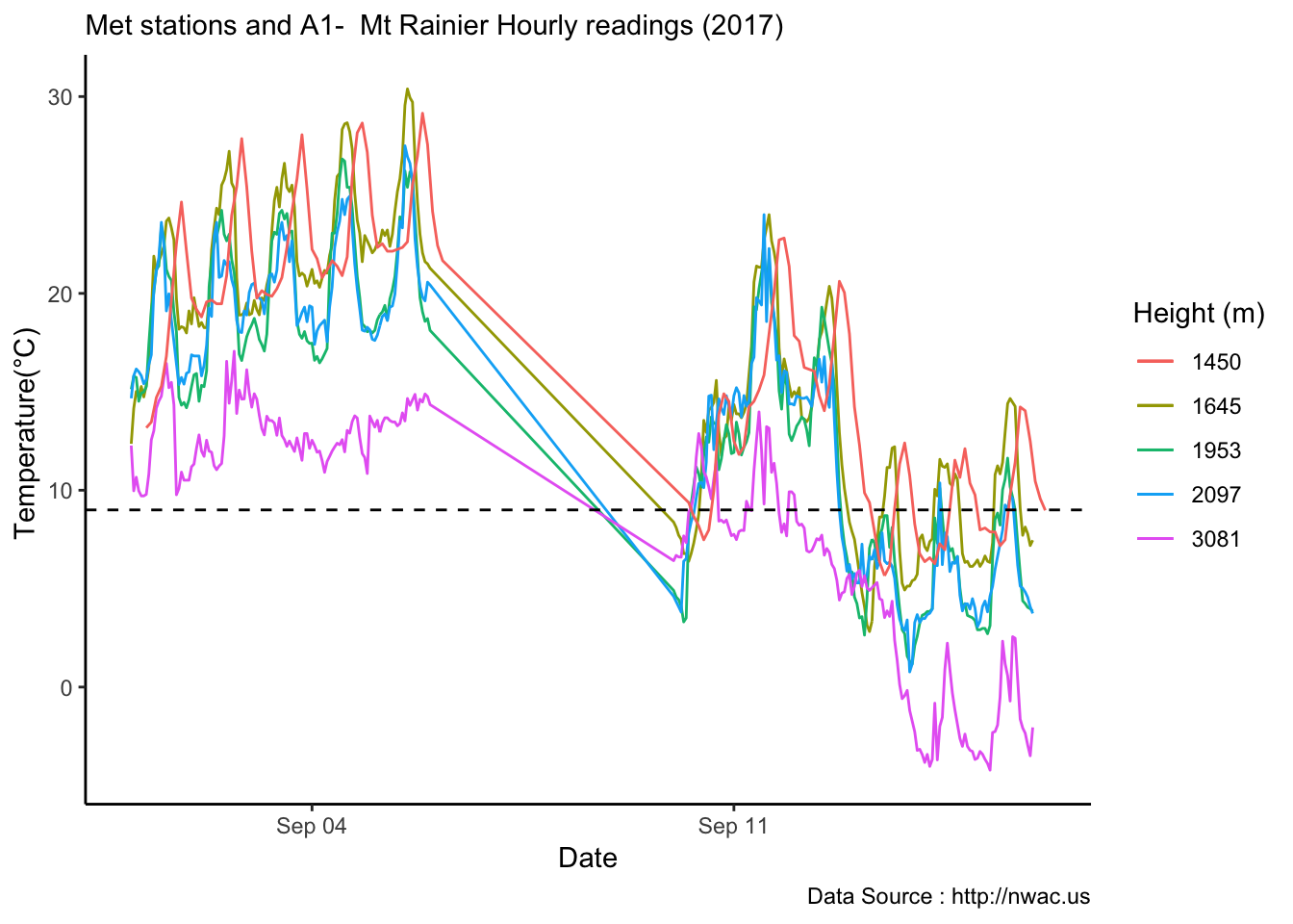
Combine whole month with A1 2017
# read in Paradise
MtRainier_Local_2017 %>% filter(year== 2017) %>%
ggplot() +
geom_line(aes(datetime,weathermetrics::fahrenheit.to.celsius(Paradise_5400),col='1645')) +
geom_line(aes(datetime,weathermetrics::fahrenheit.to.celsius(Sunrise_6410),col='1953')) +
geom_line(aes(datetime,weathermetrics::fahrenheit.to.celsius(Sunrise_6880),col='2097')) +
geom_line(aes(datetime,weathermetrics::fahrenheit.to.celsius(CampMuir_10110),col='3081')) +
geom_line(data=MtRainier_AE10A1_1718[MtRainier_AE10A1_1718$year== 2017 ,],aes(timect,Temp,col='1450')) +
theme_classic() + labs(x="Date", y="Temperature(°C) ", color = "Height (m)",
subtitle="Met stations and A1- Mt Rainier Hourly readings (2017) ", caption="Data Source : http://nwac.us") +
geom_hline(aes(yintercept=9),colour="black", linetype="dashed") 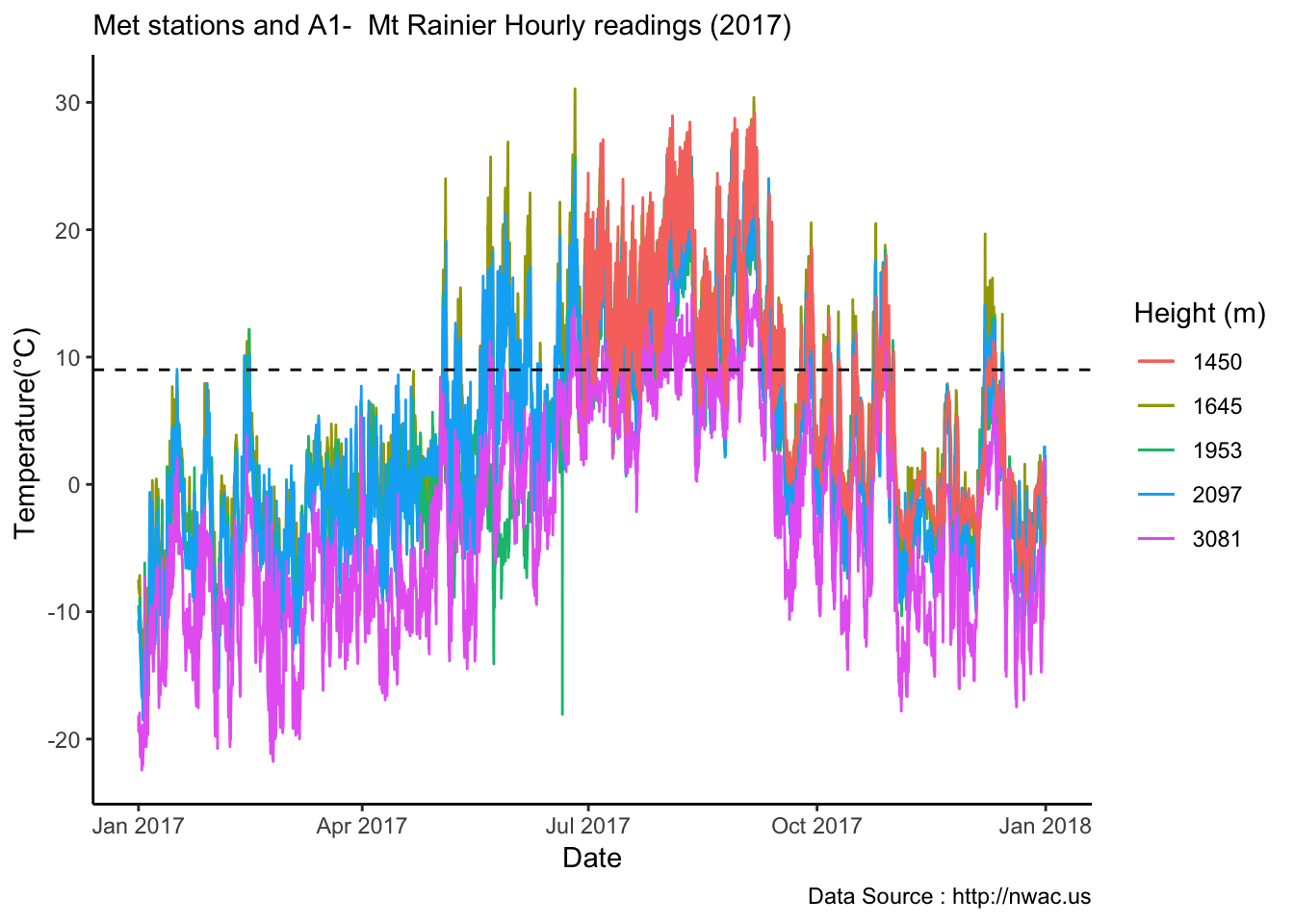 ## 1-04-2019
Plotting the min and max of the coop and snotel
MtRainier_coopsnowsep_longmire <- read_csv('./data/UCC_ghcn_Longmire.csv',comment = '#')## Parsed with column specification:
## cols(
## Day = col_date(format = ""),
## Precipitation = col_character(),
## Min_Temperature = col_character(),
## Max_Temperature = col_character()
## )MtRainier_coopsnowsep_skatecreek <- read_csv('./data/UCC_ghcn_SkateCreek.csv',comment = '#')## Parsed with column specification:
## cols(
## Day = col_date(format = ""),
## Precipitation = col_character(),
## Min_Temperature = col_character(),
## Max_Temperature = col_character()
## )MtRainier_coopsnowsep_Paradise <- read_csv('./data/UCC_ghcn_Paradise.csv',comment = '#')## Parsed with column specification:
## cols(
## Day = col_date(format = ""),
## Precipitation = col_character(),
## Min_Temperature = col_character(),
## Max_Temperature = col_character()
## )MtRainier_coopsnowsep_longmire$day <- day(MtRainier_coopsnowsep_longmire$Day)
MtRainier_coopsnowsep_longmire$month<- month(MtRainier_coopsnowsep_longmire$Day)
MtRainier_coopsnowsep_longmire$year<- year(MtRainier_coopsnowsep_longmire$Day)
MtRainier_coopsnowsep_longmire %>%
filter(year== 2018) %>%
ggplot() +
geom_line(aes(Day,as.numeric(Min_Temperature),col='1')) +
geom_line(aes(Day,as.numeric(Max_Temperature),col='2')) +
geom_line(data=MtRainier_coopsnowsep_skatecreek,aes(Day,as.numeric(Min_Temperature),col='3')) +
geom_line(data=MtRainier_coopsnowsep_skatecreek,aes(Day,as.numeric(Max_Temperature),col='4')) +
geom_line(data=MtRainier_coopsnowsep_Paradise,aes(Day,as.numeric(Min_Temperature),col='5')) +
geom_line(data=MtRainier_coopsnowsep_Paradise,aes(Day,as.numeric(Max_Temperature),col='6')) +
theme_classic() + labs(x="Date", y="Temperature(°C) ",subtitle="Coop/Snotel - Mt Rainier- Minimum/Max Recorded every day (2018) ", caption="Data Source : utah state climate center") +
geom_hline(aes(yintercept=9),colour="black", linetype="dashed") +
scale_colour_manual(name = 'Heights(m)',
values =c('1','2','3','4','5','6'), labels = c('841(Longmire)-Min ','841(Longmire)-Max ','1149(Skatecreek)-Min','1149(Skatecreek)-Max',"1654(Paradise)-Min","1654(Paradise)-Max"))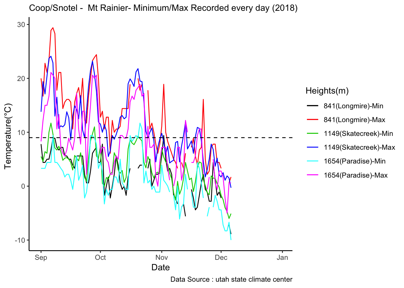
Looking at AG05 which is near Longmire
Lets look at one site
mclim_AG05_TN01_2018<- read.csv('./data/DATALOG-AG05-TN01.CSV')
names(mclim_AG05_TN01_2018) <- c('time','nodeid','temp','batt')
mclim_AG05_TN01_2018$time <- as.POSIXct(mclim_AG05_TN01_2018$time, "%Y/%m/%d %H:%M:%S")

#Add hour month and day
## 11-05-2018
mclim_AG05_TN01_2018$hr <- hour(mclim_AG05_TN01_2018$time)
mclim_AG05_TN01_2018$minute<- minute(mclim_AG05_TN01_2018$time)
mclim_AG05_TN01_2018$day <- day(mclim_AG05_TN01_2018$time)
mclim_AG05_TN01_2018$month<- month(mclim_AG05_TN01_2018$time)

#Roughly one feet apart
mclim_AG05_TN01_2018$height <- 0

mclim_AG05_TN01_2018[mclim_AG05_TN01_2018$nodeid=='28E21777910602CF' ,]$height <- 0.6
mclim_AG05_TN01_2018[mclim_AG05_TN01_2018$nodeid=='28DE0577910A02ED' ,]$height <- 1.2
mclim_AG05_TN01_2018[mclim_AG05_TN01_2018$nodeid=='2851BA7791090256' ,]$height <- 0.3
mclim_AG05_TN01_2018[mclim_AG05_TN01_2018$nodeid=='2885827791080230' ,]$height <- 0.9

## Day plot , Representive day
mclim_AG05_TN01_2018 %>% filter(month(time) %in% '9') %>%
ggplot( aes(time,temp,color = factor(height))) + geom_line() + theme_minimal() +
ggtitle("Variation in temperature at AG05- Open")  + xlab("Date") +
  ylab("Temperature (°C)") + labs(colour = "Height(m)",
subtitle="9/17/2018",caption="Data Source : http://nanoclimate.org") 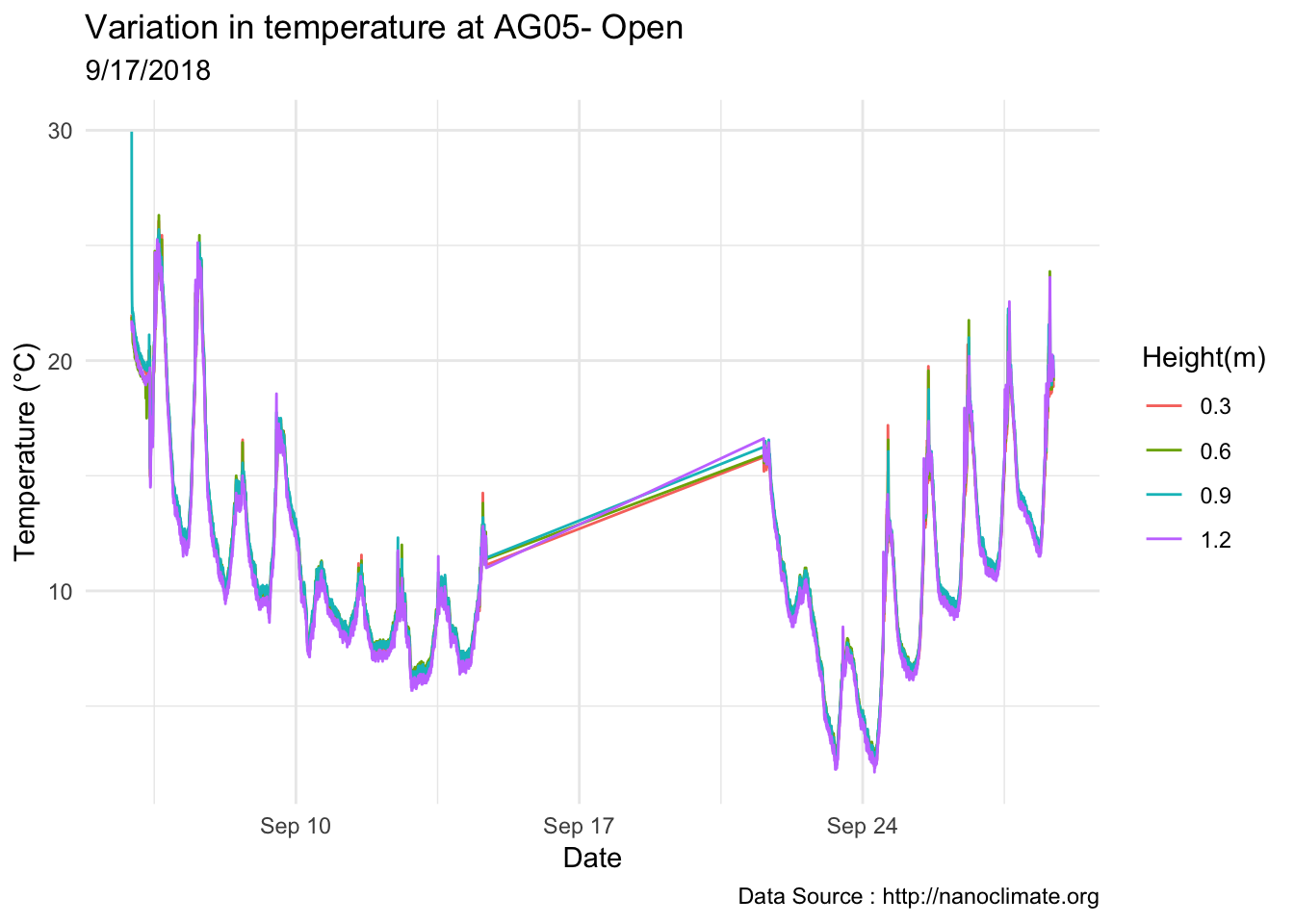
Plot Longmire and Micromet
# take height 1.2


mclim_AG05_TN01_2018 %>% filter(month(time) %in% '9' & height == 1.2) %>%
group_by(month,day) %>%
mutate(minT = min(temp),maxT=max(temp)) %>%
ggplot() +
geom_point(aes(day,minT,col='1')) +
geom_point(aes(day,maxT,col='2')) +
  geom_line(data=MtRainier_coopsnowsep_longmire[MtRainier_coopsnowsep_longmire$month==9,],aes(day,as.numeric(Min_Temperature),col='3')) +
  geom_line(data=MtRainier_coopsnowsep_longmire[MtRainier_coopsnowsep_longmire$month==9,],aes(day,as.numeric(Max_Temperature),col='4')) +
theme_minimal() +
ggtitle("Variation in temperature at AG05 TN01- Closed with Longmire")  + xlab("Date") +
  ylab("Temperature (°C)") + labs(colour = "Height(m)",
                                subtitle="",caption="Data Source : http://nanoclimate.org") +

   geom_hline(aes(yintercept=9),colour="black", linetype="dashed")  +
    scale_colour_manual(name = 'Heights(m)',
         values =c('1','2','3','4'), labels = c('MM-921(Longmire)-Min ','MM-921(Longmire)-Max ','841(Longmire)-Min','841(Longmire)-Max'))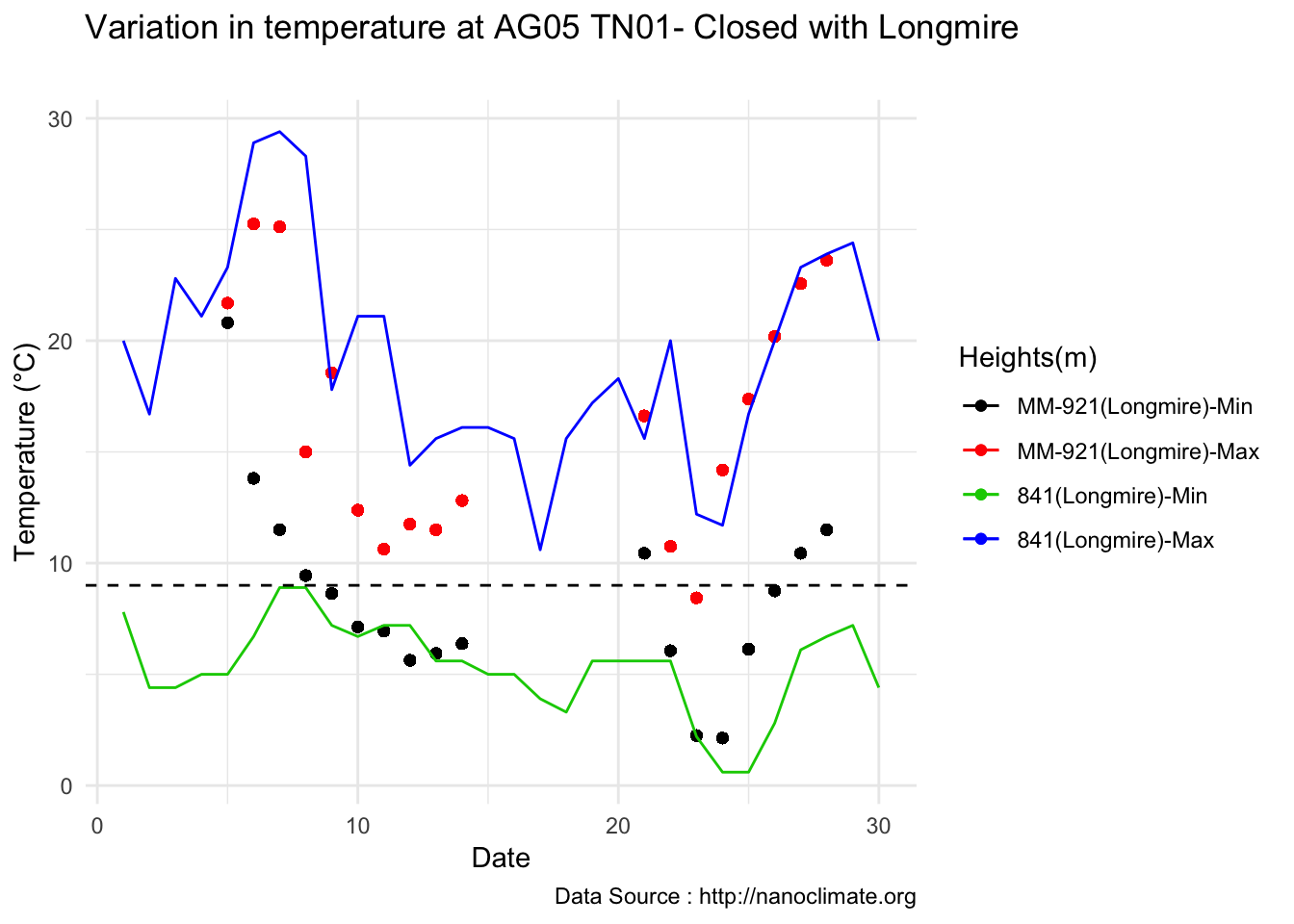
Validation
amb_4<- read_csv('./data/ambient-weather-4.csv')## Parsed with column specification:
## cols(
## .default = col_double(),
## Datetime = col_character()
## )## See spec(...) for full column specifications.amb_5<- read_csv('./data/ambient-weather-5.csv')## Parsed with column specification:
## cols(
## .default = col_double(),
## Datetime = col_character()
## )
## See spec(...) for full column specifications.amb_6<- read_csv('./data/ambient-weather-6.csv')## Parsed with column specification:
## cols(
## .default = col_double(),
## Datetime = col_character()
## )
## See spec(...) for full column specifications.amb_7<- read_csv('./data/ambient-weather-7.csv')## Parsed with column specification:
## cols(
## .default = col_double(),
## Datetime = col_character()
## )
## See spec(...) for full column specifications.amb_8<- read_csv('./data/ambient-weather-8.csv')## Parsed with column specification:
## cols(
## .default = col_double(),
## Datetime = col_character()
## )
## See spec(...) for full column specifications.amb_9<- read_csv('./data/ambient-weather-9.csv')## Parsed with column specification:
## cols(
## .default = col_double(),
## Datetime = col_character()
## )
## See spec(...) for full column specifications.amb_10<- read_csv('./data/ambient-weather-10.csv')## Parsed with column specification:
## cols(
## .default = col_double(),
## Datetime = col_character()
## )
## See spec(...) for full column specifications.amb_11<- read_csv('./data/ambient-weather-11.csv')## Parsed with column specification:
## cols(
## .default = col_double(),
## Datetime = col_character()
## )
## See spec(...) for full column specifications.amb_12<- read_csv('./data/ambient-weather-12.csv')## Parsed with column specification:
## cols(
## .default = col_double(),
## Datetime = col_character()
## )
## See spec(...) for full column specifications.amb_13<- read_csv('./data/ambient-weather-13.csv')## Parsed with column specification:
## cols(
## .default = col_double(),
## Datetime = col_character()
## )
## See spec(...) for full column specifications.amb_14<- read_csv('./data/ambient-weather-14.csv')## Parsed with column specification:
## cols(
## .default = col_double(),
## Datetime = col_character()
## )
## See spec(...) for full column specifications.amb_15<- read_csv('./data/ambient-weather-15.csv')## Parsed with column specification:
## cols(
## .default = col_double(),
## Datetime = col_character()
## )
## See spec(...) for full column specifications.amb_16<- read_csv('./data/ambient-weather-16.csv')## Parsed with column specification:
## cols(
## .default = col_double(),
## Datetime = col_character()
## )
## See spec(...) for full column specifications.amb_17<- read_csv('./data/ambient-weather-17.csv')## Parsed with column specification:
## cols(
## .default = col_double(),
## Datetime = col_character()
## )
## See spec(...) for full column specifications.amb_18<- read_csv('./data/ambient-weather-18.csv')## Parsed with column specification:
## cols(
## .default = col_double(),
## Datetime = col_character()
## )
## See spec(...) for full column specifications.amb_19<- read_csv('./data/ambient-weather-19.csv')## Parsed with column specification:
## cols(
## .default = col_double(),
## Datetime = col_character()
## )
## See spec(...) for full column specifications.amb_20<- read_csv('./data/ambient-weather-20.csv')## Parsed with column specification:
## cols(
## .default = col_double(),
## Datetime = col_character()
## )
## See spec(...) for full column specifications.amb <- bind_rows(amb_4,
amb_5,amb_6,.id = NULL)
names(amb) <- c('Datetime','Wind_Direction','Wind_Speed','Wind_Gust','Max_Daily_Gust','Outdoor_Temperature','Hourly_Rain','Event_Rain','Daily_Rain','Weekly_Rain','Monthly_Rain','Total_Rain','Relative_Pressure','Absolute_Pressure','Outdoor_Humidity','Indoor_Temperature','Indoor_Humidity','Ultra-Violet_Radiation_Index','Solar_Radiation','Feels_Like','Dew-Point')
amb$time <- as.POSIXct(amb$Datetime, format="%m/%d/%Y %I:%M %p",tz="America/Los_Angeles")
amb$hr <- hour(amb$time)
amb$minute<- minute(amb$time)
amb$day <- day(amb$time)
amb$month<- month(amb$time)
amb %>%
ggplot() +
geom_point(aes(time,Outdoor_Temperature ,col='1')) +
geom_line(aes(time,Outdoor_Temperature)) +
theme_minimal() +
ggtitle("Variation in temperature at AG05 TN01- Closed with Longmire") + xlab("Date") +
ylab("Temperature (°C)") + labs(colour = "Height(m)",
subtitle="",caption="Data Source : http://nanoclimate.org") +
geom_hline(aes(yintercept=9),colour="black", linetype="dashed") +
scale_colour_manual(name = 'Heights(m)',
values =c('1','2','3','4'), labels = c('MM-Ambient ','MM-921(Longmire)-Max ','841(Longmire)-Min','841(Longmire)-Max'))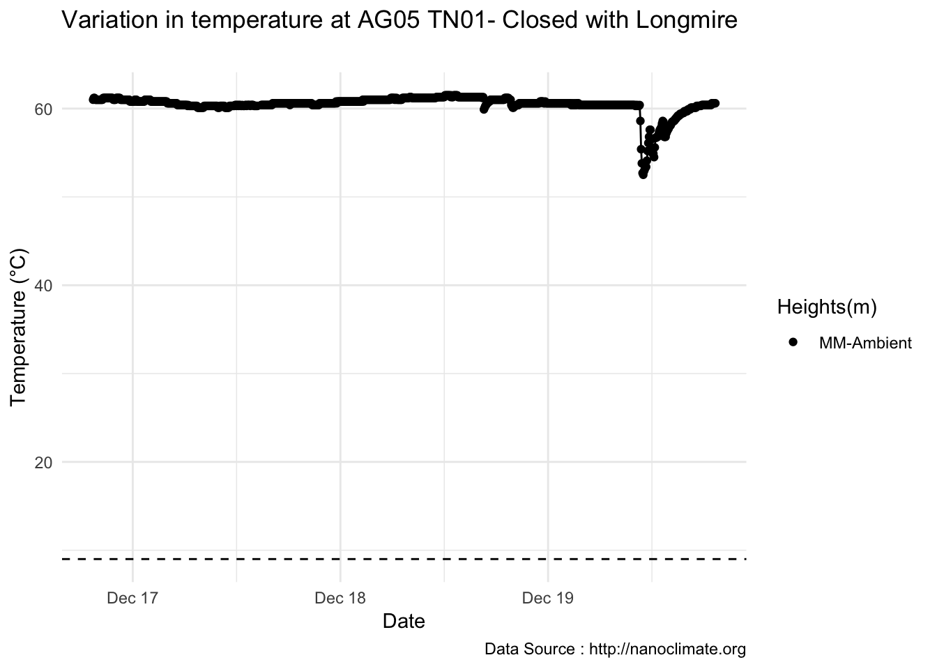
8.24 1-9-2019
Temperature profile (Diel), daily vs weekly
library(RColorBrewer)
mclim_AE10_CN01_2018 %>%  filter (!is.na(mclim_AE10_CN01_2018$minute) & month %in% c(9) ) %>%
  filter( day > 9 & day < 15)  %>%
    group_by(month,day,hr) %>%
    add_count(wt=3) %>%
    summarise(m1= mean(temp1)) %>%
  group_by(day,hr) %>%
  ggplot() +
  geom_line(aes(hr,m1,group=day ,color=as.factor(day),linetype = '1.2'),se=F)+

  scale_colour_manual("Temperature on day", breaks = c("10","11", "12","13","14"), values = brewer.pal(5, "Set1")) +
   scale_linetype_manual("Height(m)",values=c("1.2"=1)) +
  theme_classic()  + ggtitle("Diel Variation in temperature at 1.2m at site AE10 (1450m)")  + xlab("Hour") +
  ylab("Temperature (°C)") + labs(colour = "Hour",
subtitle="9/10/18 - 9/14/19",caption="Data Source : http://www.nanoclimate.org") 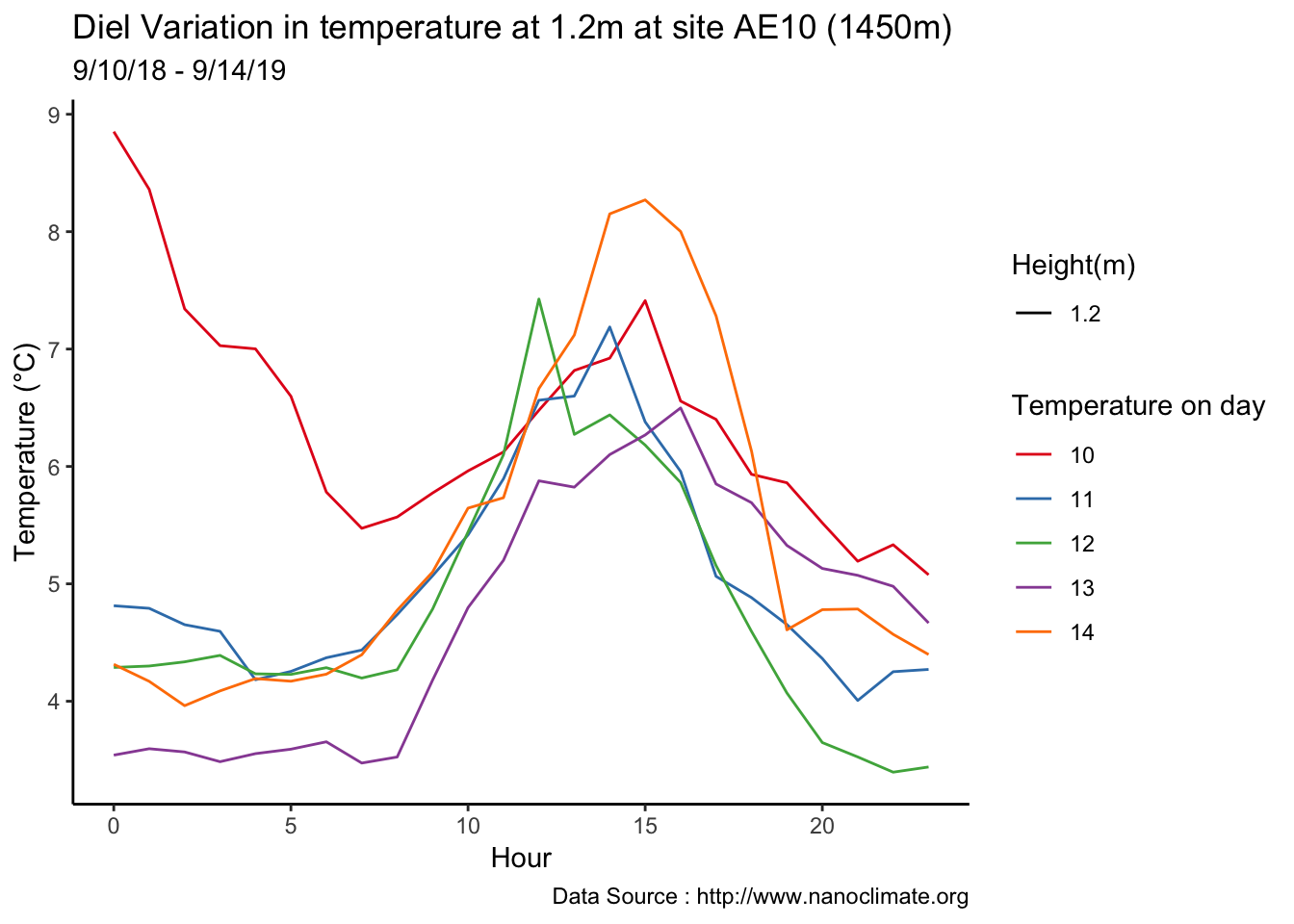
Comparing it to Paradise
library(RColorBrewer)
MtRainier_Local_2017 %>%  filter (month %in% c(9) ) %>%
  filter( day > 9 & day < 15)  %>%
    group_by(day,hr) %>%
  ggplot() +
  geom_line(aes(hr,weathermetrics::fahrenheit.to.celsius(Paradise_5400),group=day ,color=as.factor(day))) +
  scale_colour_manual("Temperature on day", breaks = c("10","11", "12","13","14"), values = brewer.pal(5, "Set1")) +
  theme_classic()  + ggtitle("Diel Variation in temperature at site Paradise (1645m) ")  + xlab("Hour") +
  ylab("Temperature (°C)") + labs(colour = "Hour",
subtitle="9/10/18 - 9/14/19",caption="Data Source : http://www.nwac.org") 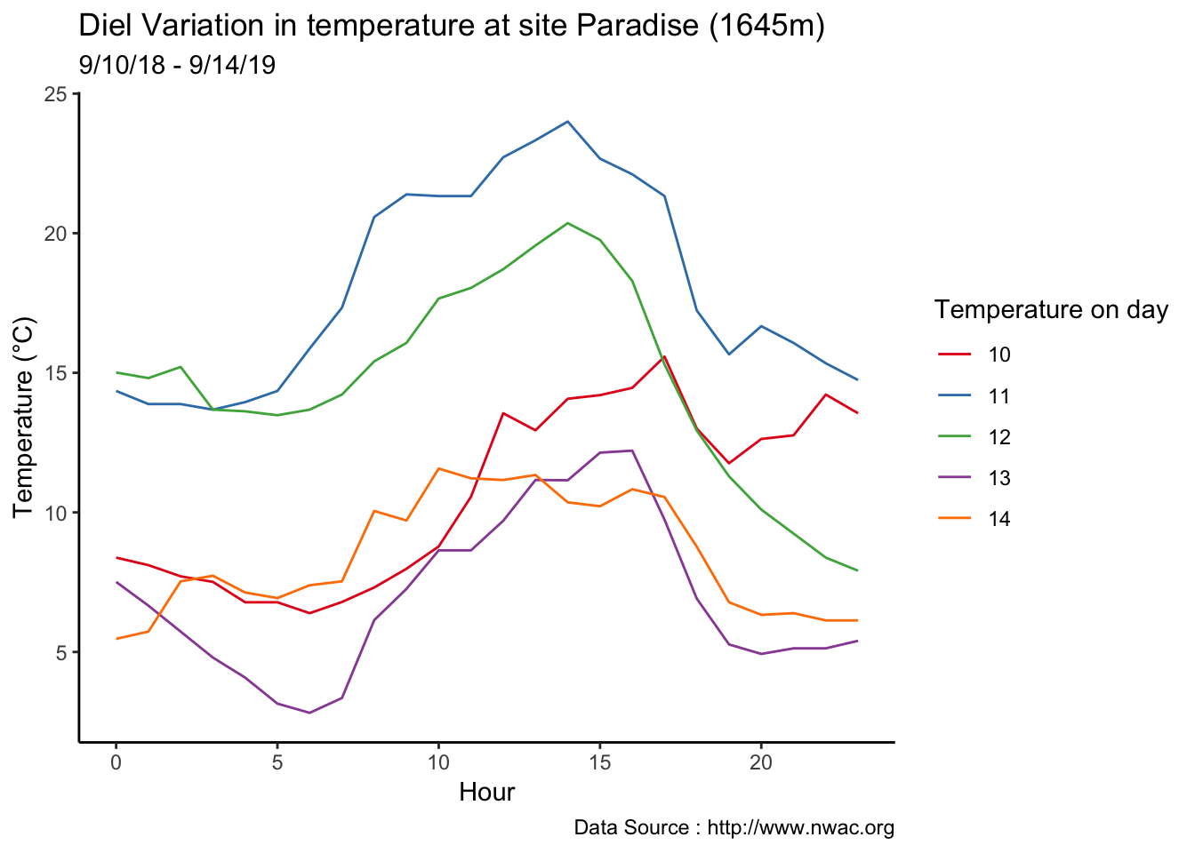
Comparing it to Sunrise Base
library(RColorBrewer)
MtRainier_Local_2017 %>%  filter (month %in% c(9) ) %>%
  filter( day > 9 & day < 15)  %>%
    group_by(day,hr) %>%
  ggplot() +
  geom_line(aes(hr,weathermetrics::fahrenheit.to.celsius(Sunrise_6410),group=day ,color=as.factor(day))) +
  scale_colour_manual("Temperature on day", breaks = c("10","11", "12","13","14"), values = brewer.pal(5, "Set1")) +
  theme_classic()  + ggtitle("Diel Variation in temperature at site Sunrise Base (1953m) ")  + xlab("Hour") +
  ylab("Temperature (°C)") + labs(colour = "Hour",
subtitle="9/10/18 - 9/14/19",caption="Data Source : http://www.nwac.org") 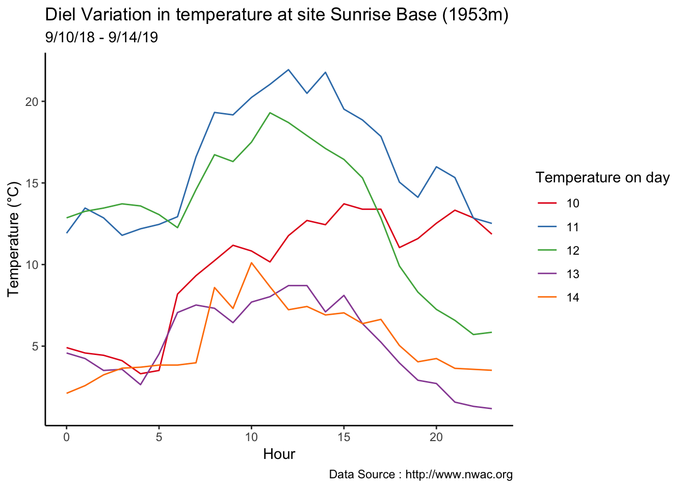
Need to add interpolated for Longmire.
Onto Radiation, use AE10-CN01
mclim_AE10_CN01_2018 %>%  filter (!is.na(mclim_AE10_CN01_2018$minute) & month %in% c(9) ) %>%
  filter( day > 9 & day < 15)  %>%
        mutate(solrf = ((solar-39) * 1.8) + ((25 -temp1) * .0012)) %>%
    group_by(month,day,hr) %>%
    add_count(wt=3) %>%
    summarise(m1= mean(solrf)) %>%
  group_by(day,hr) %>%
  ggplot() +
  geom_line(aes(hr,m1,group=day ,color=as.factor(day),linetype = '1.2'),se=F)+

  scale_colour_manual("Solar radiatiion on day", breaks = c("10","11", "12","13","14"), values = brewer.pal(5, "Set1")) +
   scale_linetype_manual("Height(m)",values=c("1.2"=1)) +
  theme_classic()  + ggtitle("Diel Variation in radiation at 1.2m at site AE10 (1450m)")  + xlab("Hour") +
  ylab("Radiation (W/m^2)") + labs(colour = "Hour",
subtitle="9/10/18 - 9/14/19",caption="Data Source : http://www.nanoclimate.org") 
Paradise radiation
MtRainier_Solar %>% filter(month == 9 & year== 2018 & day %in% c(10,11,12,13,14) ) %>%
  ggplot() +
  geom_line(aes(hr,Paradise_5400,group=day ,color=as.factor(day))) +
  scale_colour_manual("Solar radiatiion on day", breaks = c("10","11", "12","13","14"), values = brewer.pal(5, "Set1")) +
  scale_x_continuous(breaks = c(seq(0,23,by=1))) +
   theme_classic() + labs(x="Date", y="Solar radiation(W/m2) ",subtitle="Met station Paradise (1645m) -  Mt Rainier  Solar ",                                                                                                   caption="Data Source : http://nanoclimate.org") +
geom_hline(aes(yintercept=9),colour="black", linetype="dashed") 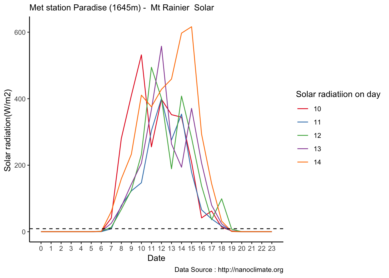
MtRainier_Solar %>% filter(month == 9 & year== 2018 & day %in% c(10,11,12,13,14) ) %>%
  ggplot() +
  geom_line(aes(hr,Sunrise_6880,group=day ,color=as.factor(day))) +
  scale_colour_manual("Solar radiatiion on day", breaks = c("10","11", "12","13","14"), values = brewer.pal(5, "Set1")) +
   theme_classic() + labs(x="Date", y="Solar radiation(W/m2) ",subtitle="Met station Sunrise base (2097m) -  Mt Rainier  Solar ",                                                                                                   caption="Data Source : http://nanoclimate.org") +
geom_hline(aes(yintercept=9),colour="black", linetype="dashed") 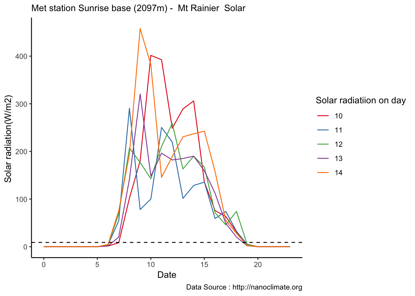
Daily solar, but average a 12 min interval.
labelsx <- c( "0","-", "-", "-", "-" ,
                "1","-", "-", "-", "-",  "2" , "-", "-", "-", "-",
                "3", "-", "-", "-", "-",  "4",  "-", "-", "-", "-",
                "5", "-", "-", "-", "-",  "6",  "-", "-", "-", "-",
                "7", "-", "-", "-", "-", "8", "-", "-", "-", "-",
                "9", "-", "-", "-", "-", "10",  "-", "-", "-", "-",
                "11", "-", "-", "-", "-", "12",  "-", "-", "-", "-",
                "13", "-", "-", "-", "-", "14",  "-", "-", "-", "-",
                "15", "-", "-", "-", "-", "16",  "-", "-", "-", "-",
                "17", "-", "-", "-", "-", "18",  "-", "-", "-", "-",
                "19", "-", "-", "-", "-", "20",  "-", "-", "-", "-",
                "21", "-", "-", "-", "-", "22",  "-", "-", "-", "-",
                "23",  "-", "-", "-", "-")
mclim_AE10_CN01_2018 %>%  filter (!is.na(mclim_AE10_CN01_2018$minute) & month %in% c(9) ) %>%
  filter( day > 9 & day < 11)  %>%
        mutate(solrf = ((solar-39) * 1.8) + ((25 -temp1) * .0012)) %>%
  group_by(hr,minute) %>%
      summarise(solmin = mean(solrf)) %>%
      group_by(b = gl(ceiling(n()/4), 4, n())) %>%
      group_by(hr,b) %>%
      summarize(meansol = mean(solmin),
                sd = sd(solmin)) %>%
      mutate(height="1.2",newx= as.numeric(paste(hr,b,sep=""))) %>%  #select(newx) %>% distinct(newx)
      dplyr::group_by(height) %>%
      mutate(index=1:n()) %>%

  ggplot() +
  geom_line(aes(index,meansol))+
        theme_minimal() +
      scale_x_continuous(breaks = seq(0,119,by=1), limits = c(0,120),labels = labelsx) +

  scale_colour_manual("Solar radiatiion on day", breaks = c("10","11", "12","13","14"), values = brewer.pal(5, "Set1")) +
   scale_linetype_manual("Height(m)",values=c("1.2"=1)) +
  theme_classic()  + ggtitle("Diel Variation in radiation at 1.2m at site AE10")  + xlab("Hour") +
  ylab("Radiation (W/m^2)") + labs(colour = "Hour",
subtitle="9/10/18 - 9/14/19",caption="Data Source : http://www.nanoclimate.org") 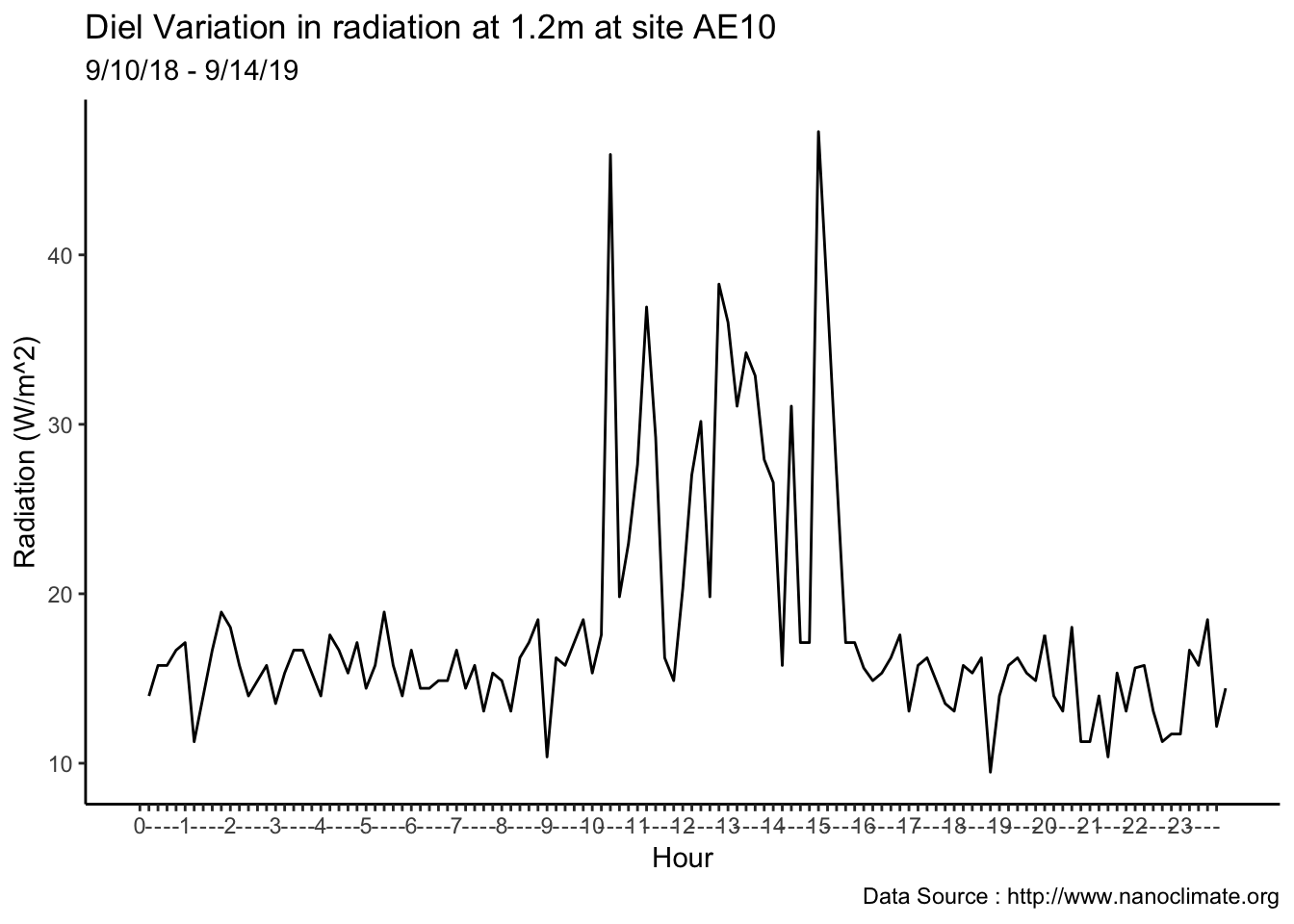
8.25 1-10-2019
Combining the plots onto a single plot
Create three dataframes to combine into one
MtRainier_Local_2018<- read_csv('./data/mt-rainier_temperature_2018.csv')## Parsed with column specification:
## cols(
## `Date/Time (PST)` = col_datetime(format = ""),
## `deg F - 5400' - Paradise` = col_double(),
## `deg F - 6410' - Sunrise Base` = col_double(),
## `deg F - 6880' - Sunrise Upper` = col_double(),
## `deg F - 10110' - Camp Muir` = col_double()
## )colnames(MtRainier_Local_2018) <- c('datetime','Paradise_5400','Sunrise_6410','Sunrise_6880','CampMuir_10110')
MtRainier_Local_2018$hr <- hour(MtRainier_Local_2018$datetime)
MtRainier_Local_2018$minute <- minute(MtRainier_Local_2018$datetime)
MtRainier_Local_2018$day <- day(MtRainier_Local_2018$datetime)
MtRainier_Local_2018$month<- month(MtRainier_Local_2018$datetime)
MtRainier_Local_2018$year<- year(MtRainier_Local_2018$datetime)
#subset dataframe for AE 10
ae1010to14 <- mclim_AE10_CN01_2018 %>% filter (!is.na(mclim_AE10_CN01_2018$minute) & month %in% c(9) ) %>%
filter( day > 9 & day < 15) %>%
group_by(month,day,hr) %>%
add_count(wt=3) %>%
summarise(m1= mean(temp1)) %>%
group_by(day,hr) %>% as.data.frame()
ae1010to14$site <- 'AE10'
Paradise_10to14 <- MtRainier_Local_2018 %>% filter (month %in% c(9) ) %>%
filter( day > 9 & day < 15) %>% mutate(m1=weathermetrics::fahrenheit.to.celsius(Paradise_5400) ) %>%
group_by(month,day,hr) %>%
dplyr::select(month,day,hr,m1) %>% as.data.frame()
Paradise_10to14$site <- 'Paradise_5400'
Sunrise_10to14 <- MtRainier_Local_2018 %>% filter (month %in% c(9) ) %>%
filter( day > 9 & day < 15) %>% mutate(m1=weathermetrics::fahrenheit.to.celsius(Sunrise_6880) ) %>%
group_by(month,day,hr) %>%
dplyr::select(month,day,hr,m1) %>% as.data.frame()
Sunrise_10to14$site <- 'Sunrise_6880'
combined_10to14 <- rbind(ae1010to14,Paradise_10to14,Sunrise_10to14)Do the plot
combined_10to14 %>%  filter (month %in% c(9) ) %>%
  filter( day %in% c(10) ) %>%
    ggplot() +
  geom_line(aes(hr,m1,group=site,linetype = site),se=F)+
   scale_linetype_manual("Site(m)",values=c("AE10"=1,"Paradise_5400"=2,"Sunrise_6880"=3)) +
  theme_classic()  + ggtitle("Variation in temperature at two different heights at AE10")  + xlab("Hour") +
  ylab("Temperature (°C)") + labs(colour = "Hour",
subtitle="9/10/18",caption="Data Source : http://www.nanoclimate.org") 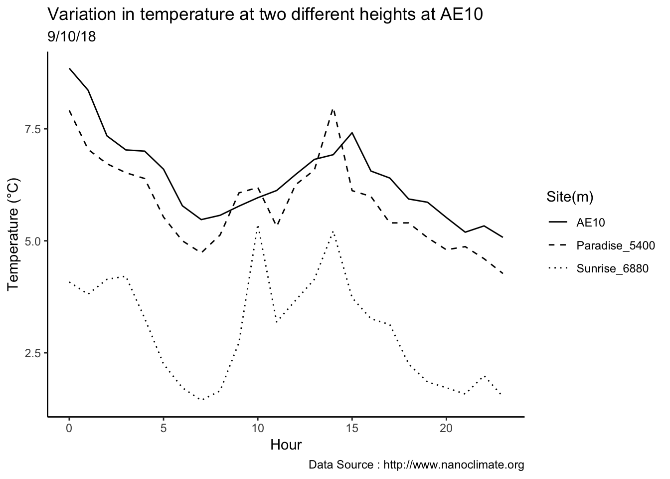
8.26 1-11-2019
Grid plots for multiple days
combined_10to14 %>%  filter (month %in% c(9) ) %>%
  filter( day %in% c(10,11,12,13,14) ) %>%
    ggplot() +
  geom_line(aes(hr,m1,group=site,linetype = site),se=F)+
  facet_grid(. ~ day) +
   scale_linetype_manual("Site(m)",values=c("AE10"=1,"Paradise_5400"=2,"Sunrise_6880"=3)) +
  theme_classic()  + ggtitle("Diel variation at differmt sites in comparion to micromet")  + xlab("Hour") +
  ylab("Temperature (°C)") + labs(colour = "Hour",
subtitle="9/10/18",caption="Data Source : http://www.nanoclimate.org") 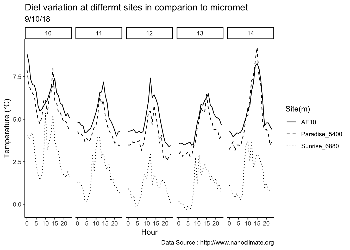
Grid for two weeks
ae10_5to15 <- mclim_AE10_CN01_2018 %>%  filter (!is.na(mclim_AE10_CN01_2018$minute) & month %in% c(9) ) %>%
  filter( day > 4 & day < 16)  %>%
    group_by(month,day,hr) %>%
    add_count(wt=3) %>%
    summarise(m1= mean(temp1)) %>%
  group_by(day,hr) %>%  as.data.frame()
ae10_5to15$site <- 'AE10_1450'

Paradise_5to15 <- MtRainier_Local_2018 %>%  filter (month %in% c(9) ) %>%
  filter( day > 4 & day < 16)   %>% mutate(m1=(Paradise_5400 - 32) * (5/9)) %>%
    group_by(month,day,hr) %>%
    dplyr::select(month,day,hr,m1) %>% as.data.frame()


Paradise_5to15$site <- 'Paradise_1645'

Sunrise_5to15 <- MtRainier_Local_2018 %>%  filter (month %in% c(9) ) %>%
  filter( day > 4 & day < 16)  %>% mutate(m1= weathermetrics::fahrenheit.to.celsius(Sunrise_6880)) %>%
    group_by(month,day,hr) %>%
    dplyr::select(month,day,hr,m1) %>% as.data.frame()

Sunrise_5to15$site <- 'Sunrise_2097'

combined_5to15  <- rbind(ae10_5to15,Paradise_5to15,Sunrise_5to15)


combined_5to15 %>%  filter (month %in% c(9) ) %>%
  filter( day %in% c(5,6,7,8,9,10,11,12,13,14) ) %>%
    ggplot() +
  geom_line(aes(hr,m1,group=site,linetype = site),se=F)+
  facet_grid(. ~ day, scales = "free") +
   scale_linetype_manual("Site(m)",values=c("AE10_1450"=1,"Paradise_1645"=2,"Sunrise_2097"=3)) +
  theme_classic()  + ggtitle("Diel variation in Temperature at different sites in comparison to micromet")  + xlab("Hour") +
  ylab("Temperature (°C)") + labs(colour = "Hour",
subtitle="1 hr resolution",caption="Data Source : http://www.nanoclimate.org") 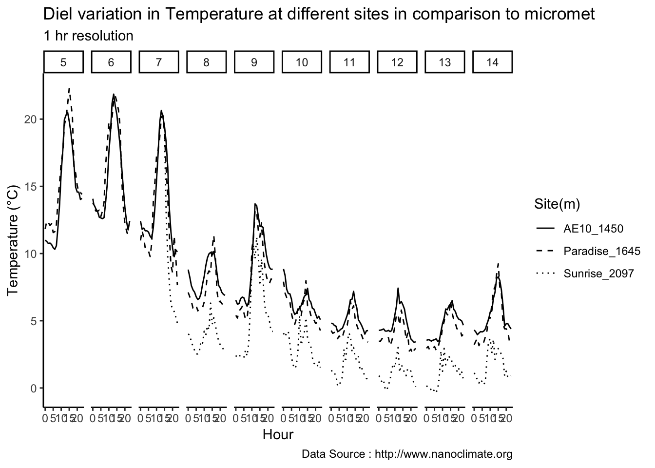
Combine Solar radiation
ae10_5to15_solar <-  mclim_AE10_CN01_2018 %>%  filter (!is.na(mclim_AE10_CN01_2018$minute) & month %in% c(9) ) %>%
  filter( day > 4 & day < 16)  %>%
        mutate(solrf = ((solar-39) * 1.8) + ((25 -temp1) * .0012)) %>%
    group_by(month,day,hr) %>%
    add_count(wt=3) %>%
    summarise(m1= mean(solrf)) %>%
  group_by(day,hr) %>%  as.data.frame()


ae10_5to15_solar$site <- 'AE10_1450'

Paradise_5to15_solar <- MtRainier_Solar %>%  filter (month %in% c(9) ) %>%
  filter( day > 4 & day < 16)  %>%
    group_by(month,day,hr) %>%
    summarise(m1= mean(Paradise_5400)) %>%
    dplyr::select(month,day,hr,m1) %>% as.data.frame()


Paradise_5to15_solar$site <- 'Paradise_1645'

Sunrise_5to15_solar <- MtRainier_Solar %>%  filter (month %in% c(9) ) %>%
  filter( day > 4 & day < 16)  %>%
    group_by(month,day,hr) %>%
    summarise(m1= mean(Sunrise_6880)) %>%
    dplyr::select(month,day,hr,m1) %>% as.data.frame()

Sunrise_5to15_solar$site <- 'Sunrise_2097'

combined_5to15_solar  <- rbind(ae10_5to15_solar,Paradise_5to15_solar,Sunrise_5to15_solar)


combined_5to15_solar %>%  filter (month %in% c(9) ) %>%
  filter( day %in% c(5,6,7,8,9,10,11,12,13,14) ) %>%
    ggplot() +
  geom_line(aes(hr,m1,group=site,linetype = site),se=F)+
  facet_grid(. ~ day, scales = "free") +
   scale_linetype_manual("Site(m)",values=c("AE10_1450"=1,"Paradise_1645"=2,"Sunrise_2097"=3)) +
  theme_classic()  + ggtitle("Diel variation Solar radiation at different sites in comparison to micromet")  + xlab("Hour") +
  ylab("Solar radiation(W/m2)") + labs(colour = "Hour",
subtitle="1 hr resolution",caption="Data Source : http://www.nanoclimate.org") 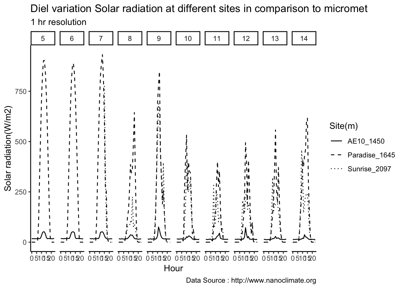
10 to 14th of September
combined_5to15_solar %>%  filter (month %in% c(9) ) %>%
  filter( day %in% c(10,11,12,13,14) ) %>%
    ggplot() +
  geom_line(aes(hr,m1,group=site,linetype = site),se=F)+
  facet_grid(. ~ day, scales = "free") +
   scale_linetype_manual("Site(m)",values=c("AE10"=1,"Paradise_5400"=2,"Sunrise_6880"=3)) +
  theme_classic()  + ggtitle("Diel variation at differmt sites in comparion to micromet")  + xlab("Hour") +
  ylab("Solar radiation(W/m2)") + labs(colour = "Hour",
subtitle="",caption="Data Source : http://www.nanoclimate.org") 
Solar radiation profile at 12 min resolution
labelfx <- c( "0","", "", "", "" ,
                "1","", "", "", "" ,  "2" , "", "", "", "" ,
                "3", "", "", "", "" ,  "4",  "", "", "", "" ,
                "5", "", "", "", "",  "6",  "", "", "", "" ,
                "7", "", "", "", "" , "8", "", "", "", "" ,
                "9", "", "", "", "" , "10", "", "", "", "" ,
                "11", "", "", "", "" , "12",  "", "", "", "" ,
                "13", "", "", "", "" , "14",  "", "", "", "" ,
                "15", "", "", "", "" , "16",  "", "", "", "" ,
                "17", "", "", "", "" , "18",  "", "", "", "" ,
                "19", "", "", "", "" , "20",  "", "", "", "" ,
                "21", "", "", "", "" , "22",  "", "", "", "" ,
                "23",  "","", "", "" )

mclim_AE10_CN01_2018 %>%  filter (!is.na(mclim_AE10_CN01_2018$minute) & month %in% c(9) ) %>%
  filter( day > 4 & day < 16)  %>%
        mutate(solrf = ((solar-39) * 1.8) + ((25 -temp1) * .0012)) %>%
  group_by(day,hr,minute) %>%
      summarise(solmin = mean(solrf)) %>%
      group_by(day,b = gl(ceiling(n()/4), 4, n())) %>%
      group_by(day,hr,b) %>%
      summarize(meansol = mean(solmin),
                sd = sd(solmin)) %>%
      mutate(height="1.2",newx= as.numeric(paste(hr,b,sep=""))) %>%  #select(newx) %>% distinct(newx)
      dplyr::group_by(day,height) %>%
      mutate(index=1:n()) %>%

  ggplot() +
  geom_line(aes(hr,meansol))+
        theme_minimal() +
  facet_grid(.~ day,scales = "free") +
#      scale_x_continuous(breaks = seq(0,119,by=1), limits = c(0,120),labels = labelfx) +

  scale_colour_manual("Solar radiatiion on day", breaks = c("10","11", "12","13","14"), values = brewer.pal(5, "Set1")) +
   scale_linetype_manual("Height(m)",values=c("1.2"=1)) +
  theme_classic()  + ggtitle("Diel Variation in radiation at 1.2m at site AE10")  + xlab("Hour") +
  ylab("Radiation (W/m^2)") + labs(colour = "Hour",
subtitle="12 min resolution",caption="Data Source : http://www.nanoclimate.org") 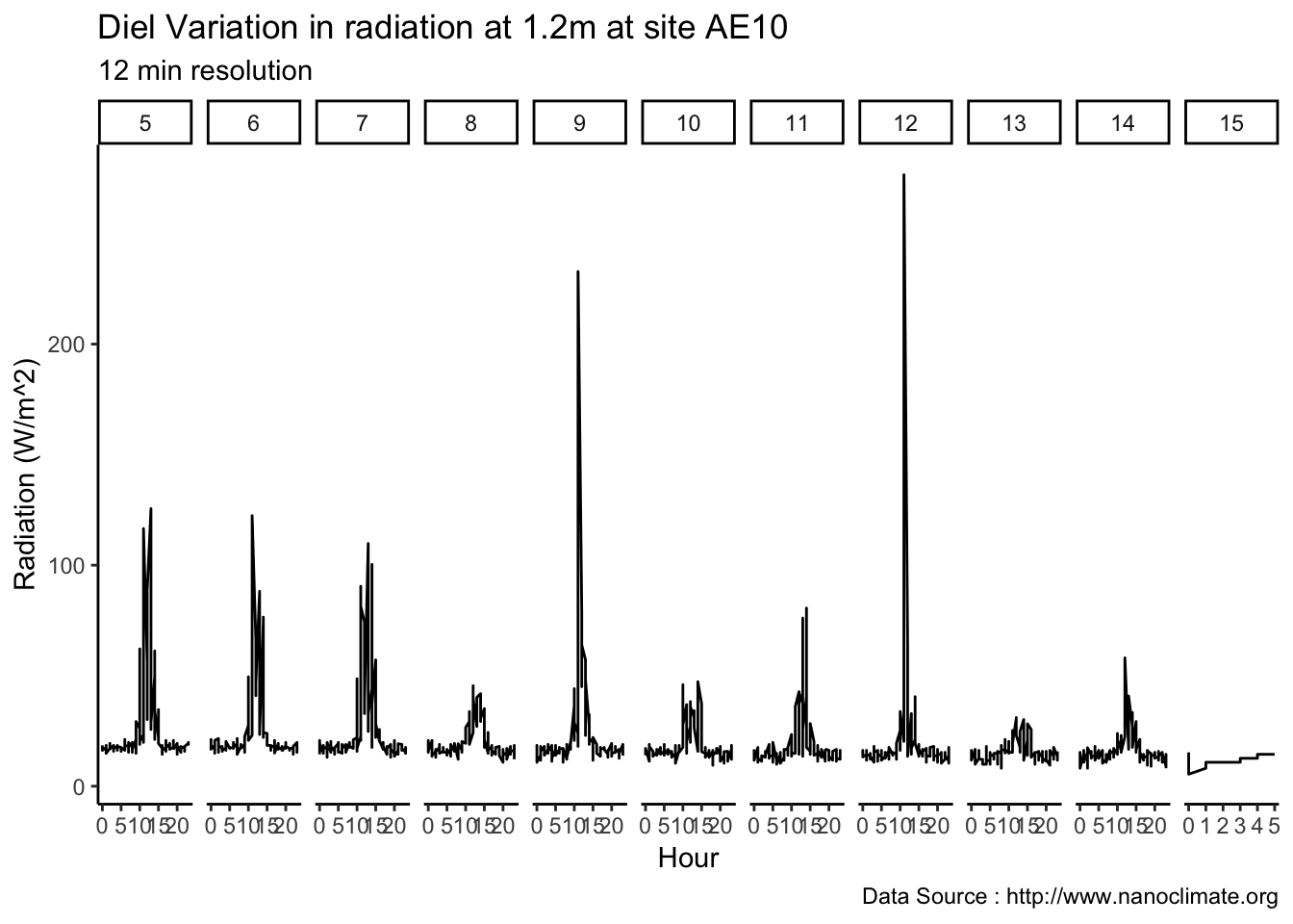
Selective plots
mclim_AE10_CN01_2018 %>%  filter (!is.na(mclim_AE10_CN01_2018$minute) & month %in% c(9) ) %>%
  filter( day > 8 & day < 13)  %>%
        mutate(solrf = ((solar-39) * 1.8) + ((25 -temp1) * .0012)) %>%
  group_by(day,hr,minute) %>%
      summarise(solmin = mean(solrf)) %>%
      group_by(day,b = gl(ceiling(n()/4), 4, n())) %>%
      group_by(day,hr,b) %>%
      summarize(meansol = mean(solmin),
                sd = sd(solmin)) %>%
      mutate(height="1.2",newx= as.numeric(paste(hr,b,sep=""))) %>%  #select(newx) %>% distinct(newx)
      dplyr::group_by(day,height) %>%
      mutate(index=1:n()) %>%

  ggplot() +
  geom_line(aes(index,meansol))+
        theme_minimal() +
  facet_grid(.~ day,scales = "free") +
      scale_x_continuous(breaks = seq(0,119,by=1), limits = c(0,120),labels = labelfx) +

  scale_colour_manual("Solar radiatiion on day", breaks = c("10","11", "12","13","14"), values = brewer.pal(5, "Set1")) +
   scale_linetype_manual("Height(m)",values=c("1.2"=1)) +
  theme_classic()  + ggtitle("Diel Variation in radiation at 1.2m at site AE10")  + xlab("Hour") +
  ylab("Radiation (W/m^2)") + labs(colour = "Hour",
subtitle="9/9/18 - 9/12/19",caption="Data Source : http://www.nanoclimate.org") 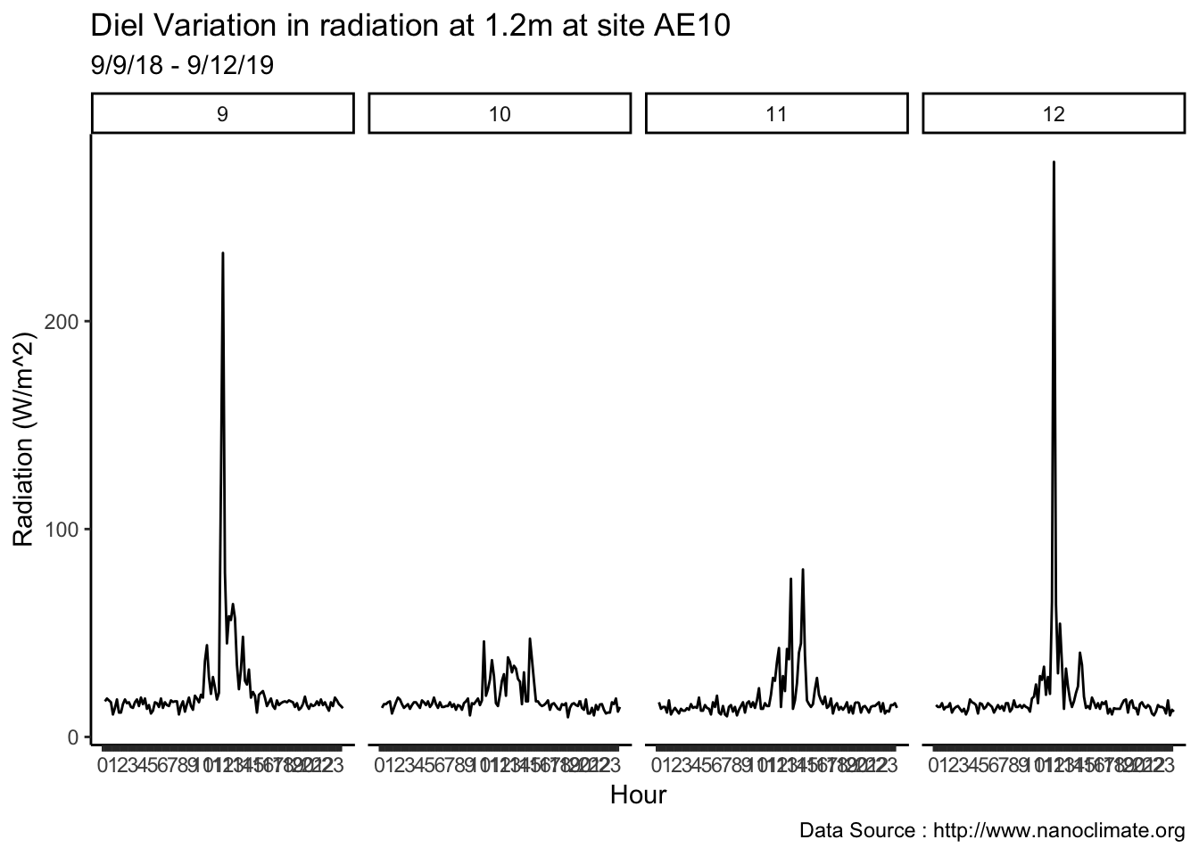
Wind profiles at 12 min resolution (0.3m)
mclim_AE10_CN01_2018 %>%  filter (!is.na(mclim_AE10_CN01_2018$minute) & month %in% c(9) ) %>%
  filter( day > 4 & day < 7)  %>%
  group_by(day,height,hr,minute) %>%
      summarise(wspd1 = mean(windspeed4)) %>%
      group_by(day,b = gl(ceiling(n()/4), 4, n())) %>%
      group_by(day,hr,b) %>%
      summarize(meanw1 = mean(wspd1),
                sd = sd(wspd1)) %>%
      mutate(ht='1.2',newx= as.numeric(paste(hr,b,sep=""))) %>%  #select(newx) %>% distinct(newx)
      dplyr::group_by(day,ht) %>%
      mutate(index=1:n()) %>%

  ggplot() +
  geom_line(aes(index,meanw1))+
        theme_minimal() +
  facet_grid(.~ day,scales = "free") +
      scale_x_continuous(breaks = seq(0,119,by=1), limits = c(0,120),labels = labelfx) +

  scale_colour_manual("Solar radiatiion on day", breaks = c("10","11", "12","13","14"), values = brewer.pal(5, "Set1")) +
   scale_linetype_manual("Height(m)",values=c("1.2"=1)) +
  theme_classic()  + ggtitle("Diel Variation in wind profile at 0.3m at site AE10")  + xlab("Hour") +
  ylab("Wind speed (km/hr)") + labs(colour = "Hour",
subtitle="12 min resolution",caption="Data Source : http://www.nanoclimate.org") 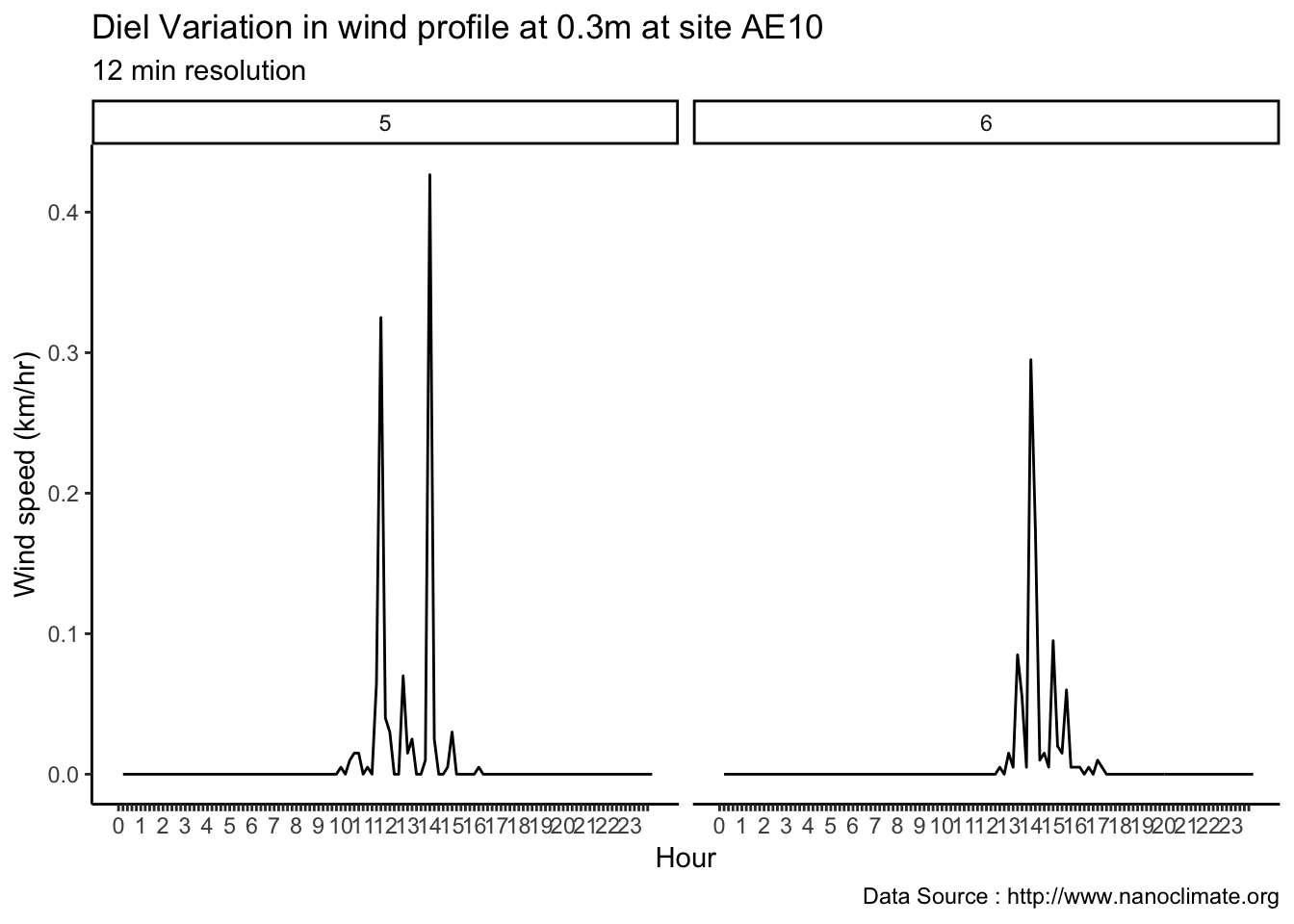
Wind profiles at 12 min resolution (0.6m)
mclim_AE10_CN01_2018 %>%  filter (!is.na(mclim_AE10_CN01_2018$minute) & month %in% c(9) ) %>%
  filter( day > 4 & day < 16)  %>%
  group_by(day,height,hr,minute) %>%
      summarise(wspd1 = mean(windspeed3)) %>%
      group_by(day,b = gl(ceiling(n()/4), 4, n())) %>%
      group_by(day,hr,b) %>%
      summarize(meanw1 = mean(wspd1),
                sd = sd(wspd1)) %>%
      mutate(ht='1.2',newx= as.numeric(paste(hr,b,sep=""))) %>%  #select(newx) %>% distinct(newx)
      dplyr::group_by(day,ht) %>%
      mutate(index=1:n()) %>%

  ggplot() +
  geom_line(aes(index,meanw1))+
        theme_minimal() +
  facet_grid(.~ day,scales = "free") +
      scale_x_continuous(breaks = seq(0,119,by=1), limits = c(0,120),labels = labelfx) +

  scale_colour_manual("Solar radiatiion on day", breaks = c("10","11", "12","13","14"), values = brewer.pal(5, "Set1")) +
   scale_linetype_manual("Height(m)",values=c("1.2"=1)) +
  theme_classic()  + ggtitle("Diel Variation in wind profile at 0.6m at site AE10")  + xlab("Hour") +
  ylab("Radiation (km/hr)") + labs(colour = "Hour",
subtitle="12 min resolution",caption="Data Source : http://www.nanoclimate.org") 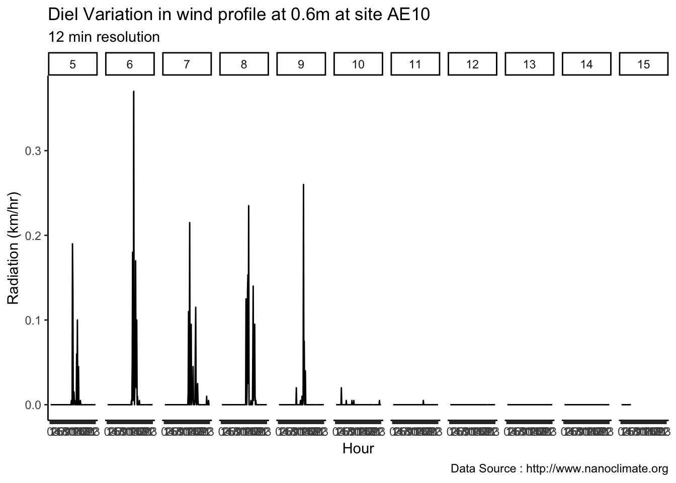
Wind profiles at 12 min resolution (0.9m)
mclim_AE10_CN01_2018 %>%  filter (!is.na(mclim_AE10_CN01_2018$minute) & month %in% c(9) ) %>%
  filter( day > 4 & day < 16)  %>%
  group_by(day,height,hr,minute) %>%
      summarise(wspd1 = mean(windspeed2)) %>%
      group_by(day,b = gl(ceiling(n()/4), 4, n())) %>%
      group_by(day,hr,b) %>%
      summarize(meanw1 = mean(wspd1),
                sd = sd(wspd1)) %>%
      mutate(ht='1.2',newx= as.numeric(paste(hr,b,sep=""))) %>%  #select(newx) %>% distinct(newx)
      dplyr::group_by(day,ht) %>%
      mutate(index=1:n()) %>%

  ggplot() +
  geom_line(aes(index,meanw1))+
        theme_minimal() +
  facet_grid(.~ day,scales = "free") +
      scale_x_continuous(breaks = seq(0,119,by=1), limits = c(0,120),labels = labelfx) +

  scale_colour_manual("Solar radiatiion on day", breaks = c("10","11", "12","13","14"), values = brewer.pal(5, "Set1")) +
   scale_linetype_manual("Height(m)",values=c("1.2"=1)) +
  theme_classic()  + ggtitle("Diel Variation in wind profile at 0.9m at site AE10")  + xlab("Hour") +
  ylab("Windspeed (km/hr)") + labs(colour = "Hour",
subtitle="12 min resolution",caption="Data Source : http://www.nanoclimate.org") 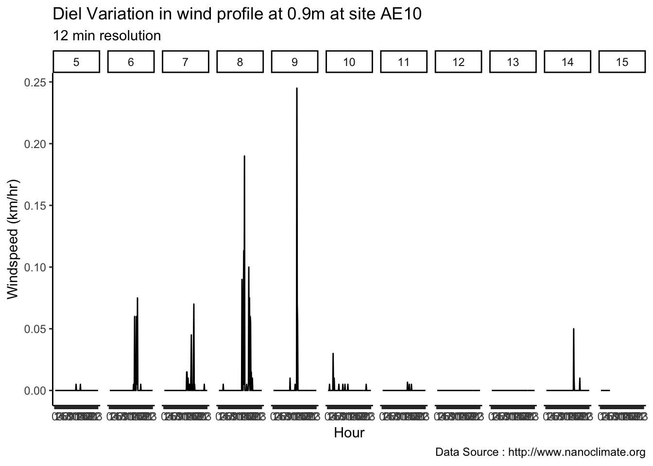
Wind profiles at 12 min resolution (1.2m)
mclim_AE10_CN01_2018 %>%  filter (!is.na(mclim_AE10_CN01_2018$minute) & month %in% c(9) ) %>%
  filter( day > 4 & day < 16)  %>%
  group_by(day,height,hr,minute) %>%
      summarise(wspd1 = mean(windspeed1)) %>%
      group_by(day,b = gl(ceiling(n()/4), 4, n())) %>%
      group_by(day,hr,b) %>%
      summarize(meanw1 = mean(wspd1),
                sd = sd(wspd1)) %>%
      mutate(ht='1.2',newx= as.numeric(paste(hr,b,sep=""))) %>%  #select(newx) %>% distinct(newx)
      dplyr::group_by(day,ht) %>%
      mutate(index=1:n()) %>%

  ggplot() +
  geom_line(aes(index,meanw1))+
        theme_minimal() +
  facet_grid(.~ day,scales = "free") +
      scale_x_continuous(breaks = seq(0,119,by=1), limits = c(0,120),labels = labelfx) +

  scale_colour_manual("Solar radiatiion on day", breaks = c("10","11", "12","13","14"), values = brewer.pal(5, "Set1")) +
   scale_linetype_manual("Height(m)",values=c("1.2"=1)) +
  theme_classic()  + ggtitle("Diel Variation in wind profile at 1.2m at site AE10")  + xlab("Hour") +
  ylab("Radiation (km/hr)") + labs(colour = "Hour",
subtitle="12 min resolution",caption="Data Source : http://www.nanoclimate.org") 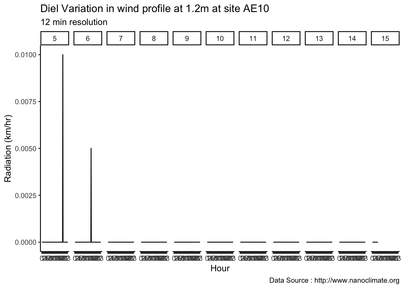
Notes from the PI meeting
Remarks
- Temperature readings from AE10 still looks very buffered (not tracking the regional)
- Solar radiation magnitude not matching-up, hard to believe canopy buffering is the cause. If canopy buffering was the case, it wont be that be that influential after the peak solar radiation.
- Battery hypothesis that being cold is making it lose the ability to capture the signal.
Next steps
- Compare with Longmire
- Compare with Skate creek and other MM sites
- If the site is buffered, previous years comparison sgould highlight that (Aji’s hypothesis), there are old-growth forests. ()
Compare with
file = 'AE10-A1_hourly.csv'

 # Read the file
   onest <- read.csv(paste("data/" , file, sep = ""))
   # Update the tumestamp
   onest$dt <- strptime(onest$DATE, format = "%Y-%m-%d %H:%M:%S")
   # add the year
   onest$year <- as.numeric(substring(as.character(onest$DATE),1,4))
   # add txn date
   onest$dt_txn <- as.POSIXct(onest$DATE,ormat = "%Y-%m-%d %H:%M:%S")
   # Add month column
   # Add day column
   # Add hour column
   onest$month <- as.numeric(format(onest$dt_txn,"%m"))
   onest$day <- as.numeric(format(onest$dt_txn,"%d"))
   onest$hr <- as.numeric(format(onest$dt,"%H"))

   onest %>%
     dplyr::select( "series_xts" ,     "year"  ,
 "dt_txn"   ,  "month"  ,    "day"  ,      "hr") %>%
     filter (month %in% c(9) ) %>%
       group_by(year,month,day,hr) %>%
    summarise(m1= mean(series_xts)) %>%
  filter( day %in% c(5,6,7,8,9) )  %>%
    ggplot() +
  geom_line(aes(hr,m1,group=as.factor(day),linetype = as.factor(day)),se=F)+
  facet_grid(. ~ year, scales = "free") +
 #  scale_linetype_manual("Site(m)",values=c("AE10_1450"=1,"Paradise_1645"=2,"Sunrise_2097"=3)) +
  theme_classic()  + ggtitle("Diel variation in Temperature at different sites in comparison to micromet")  + xlab("Hour") +
  ylab("Temperature (°C)") + labs(colour = "Hour",
subtitle="1 hr resolution",caption="Data Source : http://www.nanoclimate.org") 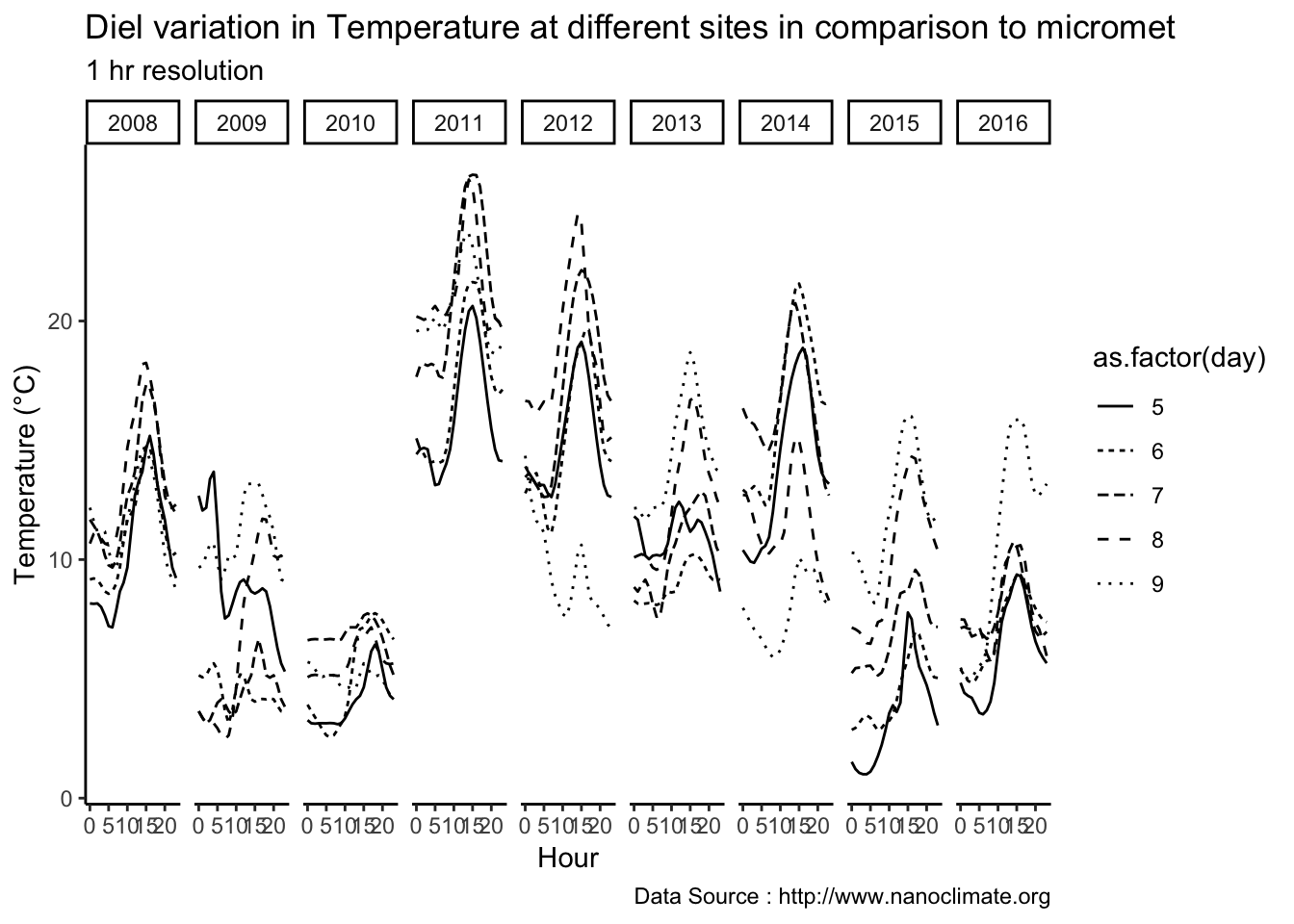
Compare 14,15 and 2016. I hypitheize that southside slope, facng tatoosh range, its a deep valley which is giving rise to the unque microclimate
Paradise_5400_2017<- read.csv('./data/Paradise_5400_feet_2017.csv')
Paradise_5400_2016<- read.csv('./data/Paradise_5400_feet_2016.csv')
Paradise_5400_2015<- read.csv('./data/Paradise_5400_feet_2015.csv')
Paradise_5400_2014<- read.csv('./data/Paradise_5400_feet_2014.csv')

Paradise_5400_2017$date <- as.Date(Paradise_5400_2017$Date.Time..PST., "%Y-%m-%d")
Paradise_5400_2017$datetime <- as.Date(Paradise_5400_2017$Date.Time..PST., "%Y-%m-%d %H:%M")
library(lubridate)
library(gridExtra)
Paradise_5400_2017$hr <-lubridate::hour(lubridate::as_datetime(Paradise_5400_2017$Date.Time..PST.))
Paradise_5400_2017$min <-lubridate::minute(lubridate::as_datetime(Paradise_5400_2017$Date.Time..PST.))
Paradise_5400_2017$month <- as.numeric (strftime(Paradise_5400_2017$Date.Time..PST.,'%m'))
Paradise_5400_2017$day <-as.numeric (strftime(Paradise_5400_2017$Date.Time..PST.,'%d'))

# 2014


Paradise_5400_2014$date <- as.Date(Paradise_5400_2014$Date.Time..PST., "%Y-%m-%d")
Paradise_5400_2014$datetime <- as.Date(Paradise_5400_2014$Date.Time..PST., "%Y-%m-%d %H:%M")
Paradise_5400_2014$hr <-lubridate::hour(lubridate::as_datetime(Paradise_5400_2014$Date.Time..PST.))
Paradise_5400_2014$min <-lubridate::minute(lubridate::as_datetime(Paradise_5400_2014$Date.Time..PST.))
Paradise_5400_2014$month <- as.numeric (strftime(Paradise_5400_2014$Date.Time..PST.,'%m'))
Paradise_5400_2014$day <-as.numeric (strftime(Paradise_5400_2014$Date.Time..PST.,'%d'))

# 2015


Paradise_5400_2015$date <- as.Date(Paradise_5400_2015$Date.Time..PST., "%Y-%m-%d")
Paradise_5400_2015$datetime <- as.Date(Paradise_5400_2015$Date.Time..PST., "%Y-%m-%d %H:%M")
Paradise_5400_2015$hr <-lubridate::hour(lubridate::as_datetime(Paradise_5400_2015$Date.Time..PST.))
Paradise_5400_2015$min <-lubridate::minute(lubridate::as_datetime(Paradise_5400_2015$Date.Time..PST.))
Paradise_5400_2015$month <-  as.numeric (strftime(Paradise_5400_2015$Date.Time..PST.,'%m'))
Paradise_5400_2015$day <- as.numeric (strftime(Paradise_5400_2015$Date.Time..PST.,'%d'))


# 2016


Paradise_5400_2016$date <- as.Date(Paradise_5400_2016$Date.Time..PST., "%Y-%m-%d")
Paradise_5400_2016$datetime <- as.Date(Paradise_5400_2016$Date.Time..PST., "%Y-%m-%d %H:%M")
Paradise_5400_2016$hr <-lubridate::hour(lubridate::as_datetime(Paradise_5400_2016$Date.Time..PST.))
Paradise_5400_2016$min <-lubridate::minute(lubridate::as_datetime(Paradise_5400_2016$Date.Time..PST.))
Paradise_5400_2016$month <-  as.numeric (strftime(Paradise_5400_2016$Date.Time..PST.,'%m'))
Paradise_5400_2016$day <- as.numeric (strftime(Paradise_5400_2016$Date.Time..PST.,'%d'))


ae10_A1_1to30_2015 <- onest %>%
     dplyr::select( "series_xts" ,     "year"  ,
 "dt_txn"   ,  "month"  ,    "day"  ,      "hr") %>%
     filter (month %in% c(9) & year ==2015) %>%
   filter(day > 0 & day < 31)  %>%
       group_by(month,day,hr) %>%
    summarise(m1= mean(series_xts)) %>%
  dplyr::select(month,day,hr,m1) %>% as.data.frame()

ae10_A1_1to30_2015$site <- 'AE10_A1_1450'

ae10_A1_1to30_2016 <- onest %>%
     dplyr::select( "series_xts" ,     "year"  ,
 "dt_txn"   ,  "month"  ,    "day"  ,      "hr") %>%
     filter (month %in% c(9) & year ==2016) %>%
   filter(day > 0 & day < 31)  %>%
       group_by(month,day,hr) %>%
    summarise(m1= mean(series_xts)) %>%
  dplyr::select(month,day,hr,m1) %>% as.data.frame()

ae10_A1_1to30_2016$site <- 'AE10_A1_1450'

Paradise_1to30_2015 <-Paradise_5400_2015 %>%  filter (month %in% c(9) ) %>%
  filter(day > 0 & day < 31)  %>%
    group_by(month,day,hr) %>%
    summarise(m1= mean(weathermetrics::fahrenheit.to.celsius(Temperature..deg.F.))) %>%
    dplyr::select(month,day,hr,m1) %>% as.data.frame()


Paradise_1to30_2015$site <- 'Paradise_2015_1645'

Paradise_1to30_2016 <-Paradise_5400_2016 %>%  filter (month %in% c(9) ) %>%
  filter(day > 0 & day < 31)  %>%
    group_by(month,day,hr) %>%
    summarise(m1= mean(weathermetrics::fahrenheit.to.celsius(Temperature..deg.F.))) %>%
    dplyr::select(month,day,hr,m1) %>% as.data.frame()


Paradise_1to30_2016$site <- 'Paradise_2016_1645'

combined_1to30_A1_2015  <- rbind(ae10_A1_1to30_2015,Paradise_1to30_2015)
combined_1to30_A1_2016  <- rbind(ae10_A1_1to30_2016,Paradise_1to30_2016)
8.27 1-12-2019
Do the comparison with year 2015 against M1
combined_1to30_A1_2015 %>%  filter (month %in% c(9) ) %>%
 # filter( day %in% c(10,11,12,13,14) ) %>%
     filter(day > 0 & day < 31)  %>%
    ggplot() +
  geom_line(aes(hr,m1,group=site,linetype = site),se=F)+
  facet_grid(. ~ day, scales = "free") +
   scale_linetype_manual("Site(m)",values=c("AE10_A1_1450"=1,"Paradise_2015_1645"=2,"Sunrise_6880"=3)) +
  theme_classic()  + ggtitle("Diel variation at different sites in comparion to A1")  + xlab("Hour") +
  ylab("Solar radiation(W/m2)") + labs(colour = "Hour",
subtitle="Year 2015",caption="Data Source : http://www.nanoclimate.org") 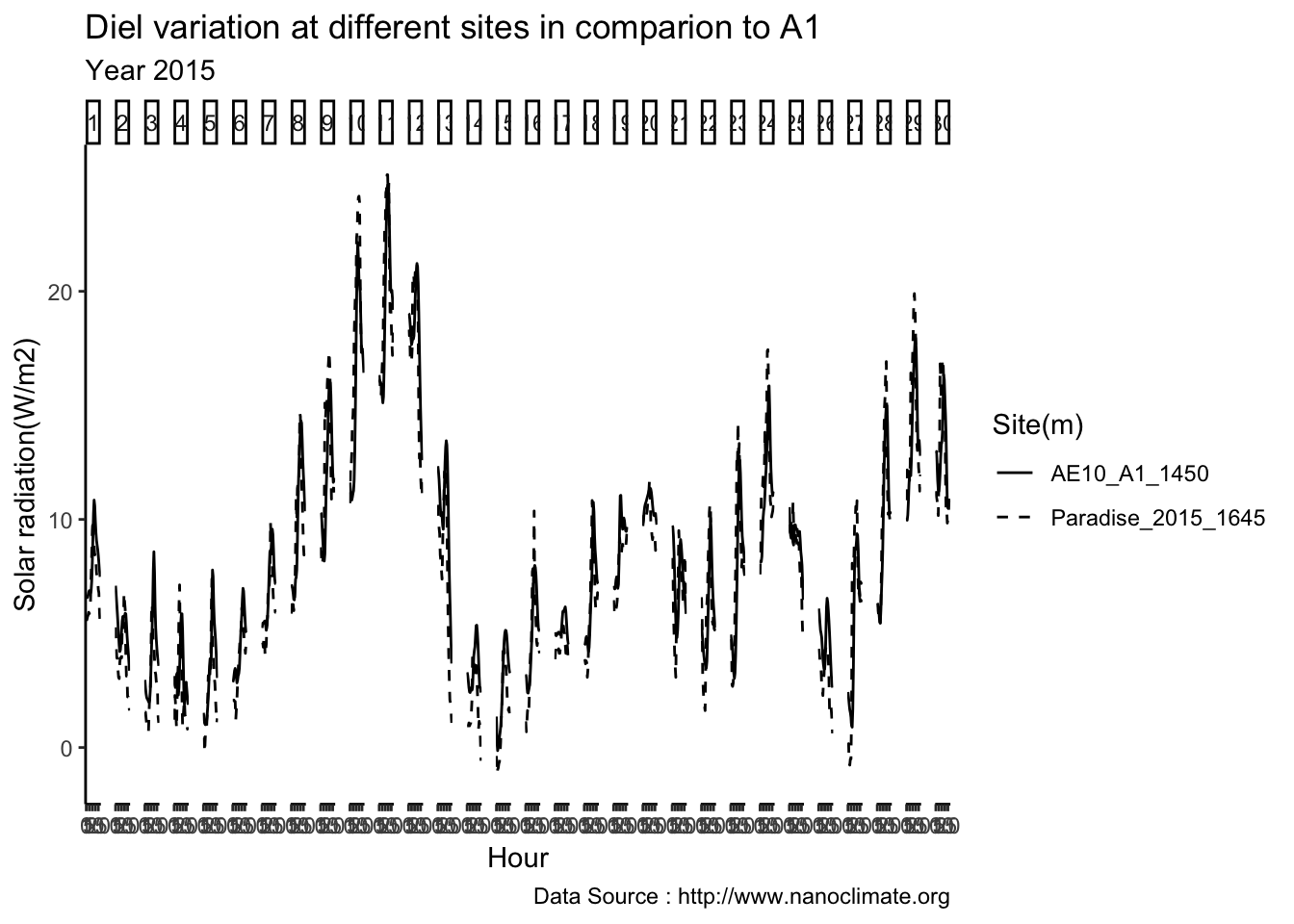
Do the comparison with year 2016 against M1
combined_1to30_A1_2016 %>%  filter (month %in% c(9) ) %>%
 # filter( day %in% c(10,11,12,13,14) ) %>%
     filter(day > 0 & day < 31)  %>%
    ggplot() +
  geom_line(aes(hr,m1,group=site,linetype = site),se=F)+
  facet_grid(. ~ day, scales = "free") +
   scale_linetype_manual("Site(m)",values=c("AE10_A1_1450"=1,"Paradise_2016_1645"=2,"Sunrise_6880"=3)) +
  theme_classic()  + ggtitle("Diel variation at different sites in comparion to A1")  + xlab("Hour") +
  ylab("Solar radiation(W/m2)") + labs(colour = "Hour",
subtitle="Year 2016",caption="Data Source : http://www.nanoclimate.org") 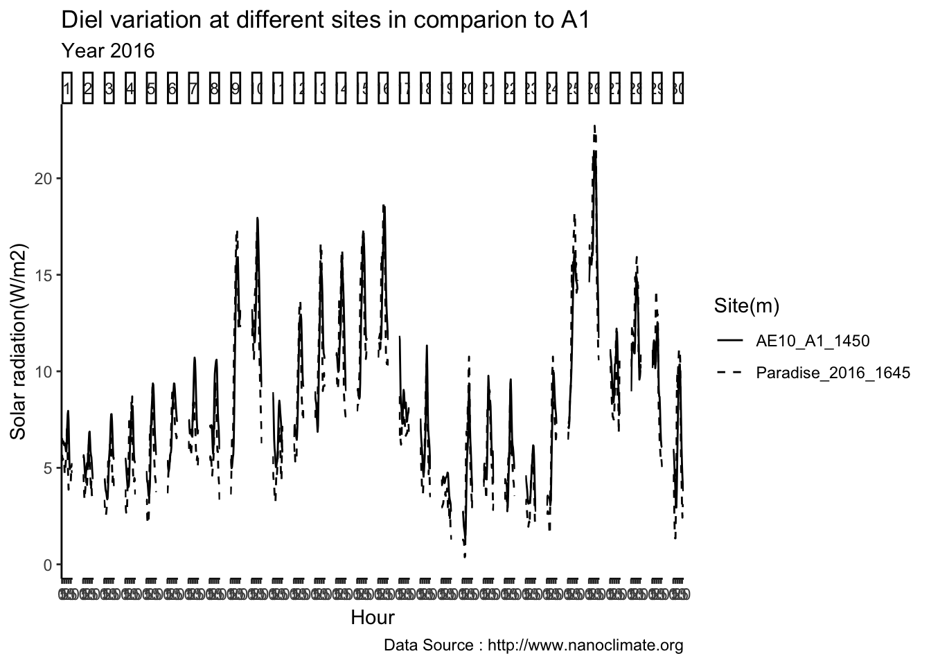
Looks like A1 is tracking quite well, adhering to principles that air temperature is quite in sync and with boundary principles, and being in the canopy does not seem to be afffecting its temperatyres .
Lets now test the hypothesis that maybe other three sites in AE10 might be capturing the signal quite well if battery is givng out.
Here I hypothesize that being in deep understory, ours should be more refglectant of the temp above ground. Inversion …..
ae10_TN01_5to15 <- mclim_AE10_TN01_2018 %>%
  filter ( month %in% c(9) & height == 0.9) %>%
  filter( day > 4 & day < 16)  %>%
    group_by(month,day,hr) %>%
    add_count(wt=3) %>%
    summarise(m1= mean(temp)) %>%
  group_by(day,hr) %>%  as.data.frame()
ae10_TN01_5to15$site <- 'AE10_TN01_1450'

ae10_TN02_5to15 <- mclim_AE10_TN02_2018 %>%
  filter (month %in% c(9) & height == 1.2) %>%
  filter( day > 4 & day < 16)  %>%
    group_by(month,day,hr) %>%
    add_count(wt=3) %>%
    summarise(m1= mean(temp)) %>%
  group_by(day,hr) %>%  as.data.frame()
ae10_TN02_5to15$site <- 'AE10_TN02_1450'

ae10_TN03_5to15 <- mclim_AE10_TN03_2018 %>%
  filter (month %in% c(9) & height == 1.2) %>%
  filter( day > 4 & day < 16)  %>%
    group_by(month,day,hr) %>%
    add_count(wt=3) %>%
    summarise(m1= mean(temp)) %>%
  group_by(day,hr) %>%  as.data.frame()
ae10_TN03_5to15$site <- 'AE10_TN03_1450'


combined_5to15_all_MMAE10  <- rbind(ae10_TN01_5to15,
                                    ae10_TN02_5to15,
                                    ae10_TN03_5to15,
                                    ae10_5to15,
                                    Paradise_5to15,
                                    Sunrise_5to15)


combined_5to15_all_MMAE10 %>%  filter (month %in% c(9) ) %>%
  filter( day %in% c(5,6,7,8,9,10,11,12,13,14) ) %>%
    ggplot() +
  geom_line(aes(hr,m1,group=site,linetype = site),se=F)+
  facet_grid(. ~ day, scales = "free") +
   scale_linetype_manual("Site(m)",values=c("AE10_TN01_1450"=1,"AE10_TN02_1450"=2,"AE10_TN03_1450"=3,"AE10_1450"=4,"Paradise_1645"=5,"Sunrise_2097"=6)) +
  theme_classic()  + ggtitle("Diel variation in Temperature at different sites in comparison to micromet")  + xlab("Hour") +
  ylab("Temperature (°C)") + labs(colour = "Hour",
subtitle="1 hr resolution",caption="Data Source : http://www.nanoclimate.org") 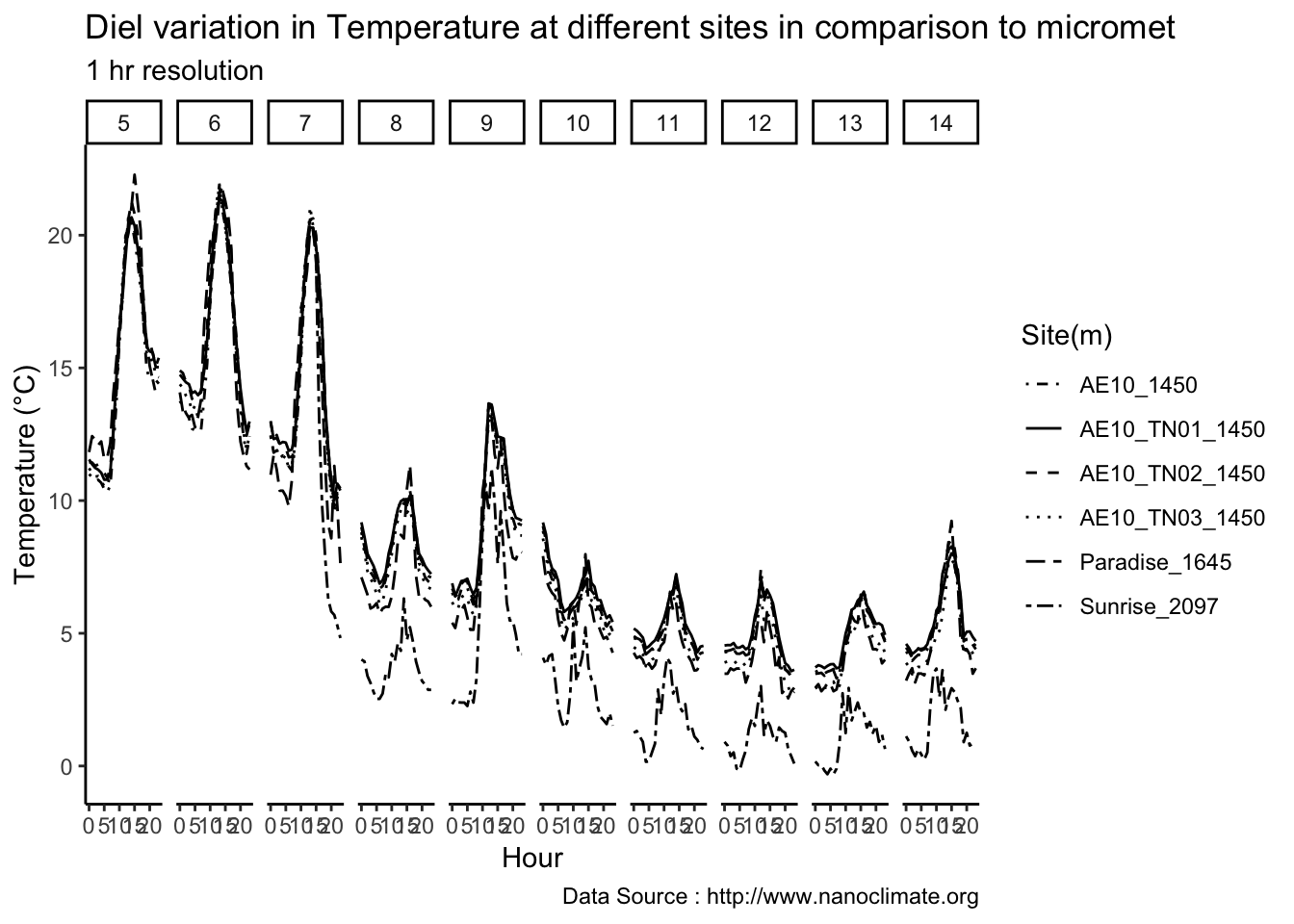
some inetersting facts, plots terrible, be selective
combined_5to15_all_MMAE10 %>%  filter (month %in% c(9) ) %>%
  filter( day %in% c(10,11,12) ) %>%
    ggplot() +
  geom_line(aes(hr,m1,group=site,linetype = site),se=F)+
  facet_grid(. ~ day, scales = "free") +
   scale_linetype_manual("Site(m)",values=c("AE10_TN01_1450"=1,"AE10_TN02_1450"=2,"AE10_TN03_1450"=3,"AE10_1450"=4,"Paradise_1645"=5,"Sunrise_2097"=6)) +
  theme_classic()  + ggtitle("Diel variation in Temperature at different sites in comparison to micromet")  + xlab("Hour") +
  ylab("Temperature (°C)") + labs(colour = "Hour",
subtitle="1 hr resolution",caption="Data Source : http://www.nanoclimate.org") 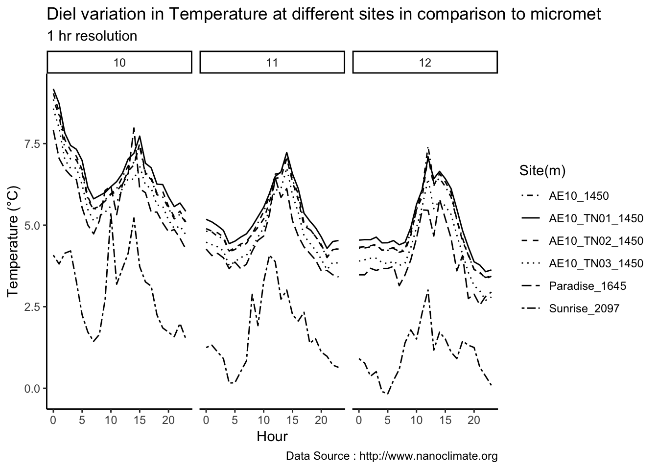
Line types not legible, lets try the color
combined_5to15_all_MMAE10 %>%  filter (month %in% c(9) ) %>%
  filter( day %in% c(5,6,7,8,9,10,11,12,13,14) ) %>%
    ggplot() +
  geom_line(aes(hr,m1,color=site),se=F)+
  facet_grid(. ~ day, scales = "free") +
   scale_color_manual("Site(m)",values=c("AE10_TN01_1450"=1,"AE10_TN02_1450"=2,"AE10_TN03_1450"=3,"AE10_1450"=4,"Paradise_1645"=5,"Sunrise_2097"=6)) +
  theme_classic()  + ggtitle("Diel variation in Temperature at different sites in comparison to micromet")  + xlab("Hour") +
  ylab("Temperature (°C)") + labs(colour = "Hour",
subtitle="1 hr resolution",caption="Data Source : http://www.nanoclimate.org") 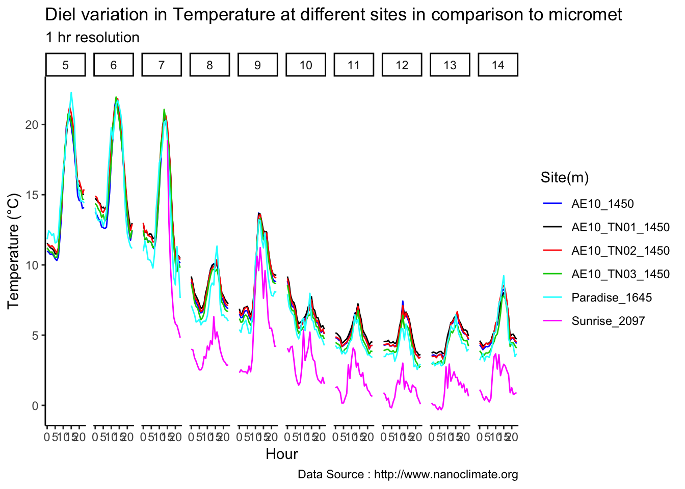
Wow, something going on, our three MM are quite inline.
combined_5to15_all_MMAE10 %>%  filter (month %in% c(9) ) %>%
  filter( day %in% c(10,11,12) ) %>%
    ggplot() +
  geom_line(aes(hr,m1,color=site),se=F)+
  facet_grid(. ~ day, scales = "free") +
   scale_color_manual("Site(m)",values=c("AE10_TN01_1450"=1,"AE10_TN02_1450"=2,"AE10_TN03_1450"=3,"AE10_1450"=4,"Paradise_1645"=5,"Sunrise_2097"=6)) +
  theme_classic()  + ggtitle("Diel variation at different sites in comparison to micromet")  + xlab("Hour") +
  ylab("Temperature (°C)") + labs(colour = "Hour",
subtitle="1 hr resolution",caption="Data Source : http://www.nanoclimate.org") 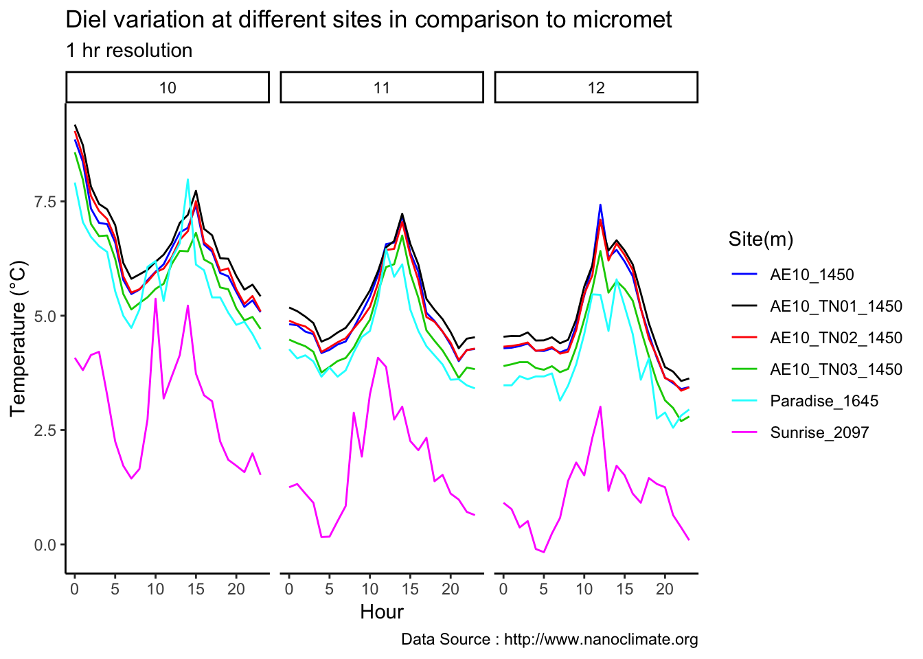
theme_Publication <- function(base_size=14, base_family="helvetica") {
      library(grid)
      library(ggthemes)
      (theme_foundation(base_size=base_size, base_family=base_family)
       + theme(plot.title = element_text(face = "bold",
                                         size = rel(1.2), hjust = 0.5),
               text = element_text(),
               panel.background = element_rect(colour = NA),
               plot.background = element_rect(colour = NA),
               panel.border = element_rect(colour = NA),
               axis.title = element_text(face = "bold",size = rel(1)),
               axis.title.y = element_text(angle=90,vjust =2),
               axis.title.x = element_text(vjust = -0.2),
               axis.text = element_text(),
               axis.line = element_line(colour="black"),
               axis.ticks = element_line(),
               panel.grid.major = element_line(colour="#f0f0f0"),
               panel.grid.minor = element_blank(),
               legend.key = element_rect(colour = NA),
               legend.position = "bottom",
               legend.direction = "horizontal",
               legend.key.size= unit(0.2, "cm"),
               legend.margin = unit(0, "cm"),
               legend.title = element_text(face="italic"),
               plot.margin=unit(c(10,5,5,5),"mm"),
               strip.background=element_rect(colour="#f0f0f0",fill="#f0f0f0"),
               strip.text = element_text(face="bold")
          ))

}
presentation_theme <- theme(axis.text = element_text(size = 25, colour = "black"),
    axis.title.x = element_text(size = 30), axis.title.y = element_text(size = 30,
        angle = 0), strip.text.x = element_text(size = 25, face = "italic"),
    strip.text.y = element_text(size = 25, angle = 270, face = "italic"), plot.title = element_text(size = 35,
        face = "bold"), legend.text = element_text(size = 20), legend.title = element_text(size = 25,
        face = "bold"))

my_theme <- theme(axis.text.x = element_text(angle = 45, vjust = 0.9,
                hjust = 0.9, size = rel(3)))
png("Spatial-MC.png",  width = 1024, height = 768, units = 'px')
combined_5to15_all_MMAE10 %>%  filter (month %in% c(9) ) %>%
  filter( day %in% c(10,11,12) ) %>%
    ggplot() +
  geom_line(aes(hr,m1,color=site),se=F)+
  facet_grid(. ~ day, scales = "free") +
   scale_color_manual("Site(m)",values=c("AE10_TN01_1450"=1,"AE10_TN02_1450"=2,"AE10_TN03_1450"=3,"AE10_1450"=4,"Paradise_1645"=5,"Sunrise_2097"=6)) +
 my_theme  + ggtitle("Diel variation at different sites in comparison to micromet")  + xlab("Hour") +
  ylab("Temperature (°C)") + labs(colour = "Hour",
                                subtitle="1 hr resolution",caption="Data Source : http://www.nanoclimate.org")
dev.off()
## quartz_off_screen
## 2Something unique,
8.28 1-15-2019
look how TN03 is the colder of them all, and also you see the tiering where TN01 and AE10 CN01 are relatively the same. This was done at .9m , so not the convential height the weater stations use.
8.29 1-16-2019
Load other stations at AG05
AG05 - TN02
Data cirruption - 9/9 from 8 pm onwards to 1am next day. 2871D7779109021D Removed the faulty record
mclim_AG05_TN02_2018<- read.csv('./data/DATALOG-AG05-TN02.CSV')
names(mclim_AG05_TN02_2018) <- c('time','nodeid','temp','batt')
mclim_AG05_TN02_2018$time <- as.POSIXct(mclim_AG05_TN02_2018$time, "%Y/%m/%d %H:%M:%S")

#Add hour month and day
## 11-05-2018
mclim_AG05_TN02_2018$hr <- hour(mclim_AG05_TN02_2018$time)
mclim_AG05_TN02_2018$minute<- minute(mclim_AG05_TN02_2018$time)
mclim_AG05_TN02_2018$day <- day(mclim_AG05_TN02_2018$time)
mclim_AG05_TN02_2018$month<- month(mclim_AG05_TN02_2018$time)

#Roughly one feet apart
mclim_AG05_TN02_2018$height <- 0

mclim_AG05_TN02_2018[mclim_AG05_TN02_2018$nodeid=='282662779114024E' ,]$height <- 0.6
mclim_AG05_TN02_2018[mclim_AG05_TN02_2018$nodeid=='28121077910602EC' ,]$height <- 1.2
mclim_AG05_TN02_2018[mclim_AG05_TN02_2018$nodeid=='2871D7779109021D' ,]$height <- 0.3
mclim_AG05_TN02_2018[mclim_AG05_TN02_2018$nodeid=='28AE157791060244' ,]$height <- 0.9

## Day plot , Representive day
mclim_AG05_TN02_2018 %>% filter(month(time) %in% '9' & day %in% c(10)) %>%
ggplot( aes(time,temp,color = factor(height))) + geom_line() + theme_minimal() +
ggtitle("Variation in temperature at AG05- TN02 Closed")  + xlab("Date") +
  ylab("Temperature (°C)") + labs(colour = "Height(m)",
subtitle="9/17/2018",caption="Data Source : http://nanoclimate.org") 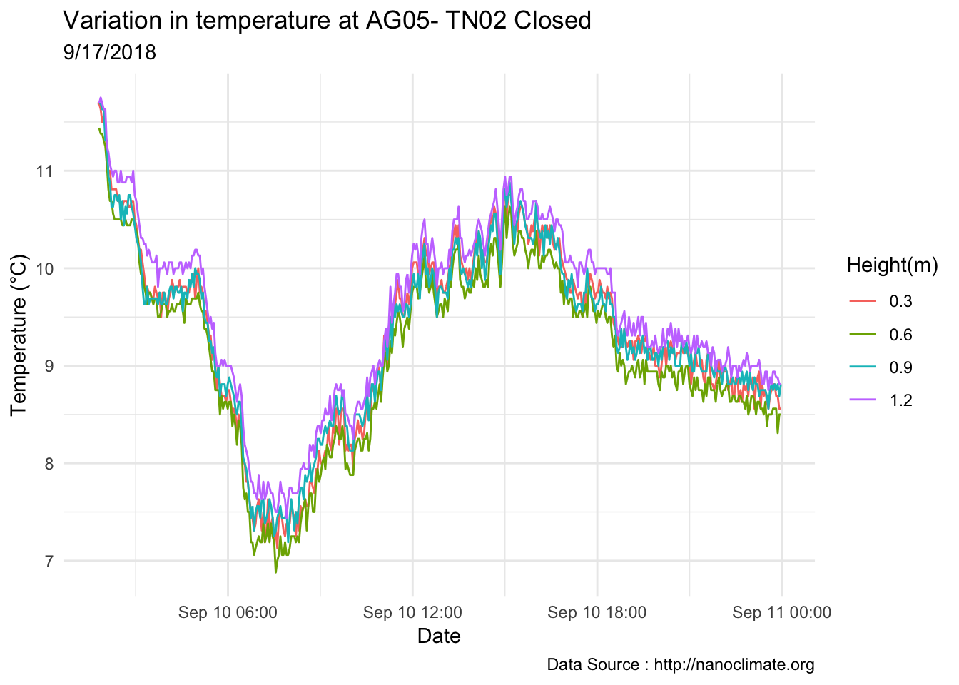
AG05 TN03
mclim_AG05_TN03_2018<- read.csv('./data/DATALOG-AG05-TN03.CSV')
names(mclim_AG05_TN03_2018) <- c('time','nodeid','temp','batt')
mclim_AG05_TN03_2018$time <- as.POSIXct(mclim_AG05_TN03_2018$time, "%Y/%m/%d %H:%M:%S")

#Add hour month and day
## 11-05-2018
mclim_AG05_TN03_2018$hr <- hour(mclim_AG05_TN03_2018$time)
mclim_AG05_TN03_2018$minute<- minute(mclim_AG05_TN03_2018$time)
mclim_AG05_TN03_2018$day <- day(mclim_AG05_TN03_2018$time)
mclim_AG05_TN03_2018$month<- month(mclim_AG05_TN03_2018$time)

#Roughly one feet apart
mclim_AG05_TN03_2018$height <- 0

mclim_AG05_TN03_2018[mclim_AG05_TN03_2018$nodeid=='282E997791080298' ,]$height <- 0.6
mclim_AG05_TN03_2018[mclim_AG05_TN03_2018$nodeid=='28A005779106022B' ,]$height <- 1.2
mclim_AG05_TN03_2018[mclim_AG05_TN03_2018$nodeid=='286EF577910A024C' ,]$height <- 0.3
mclim_AG05_TN03_2018[mclim_AG05_TN03_2018$nodeid=='2886E177910902F2' ,]$height <- 0.9

## Day plot , Representive day
mclim_AG05_TN03_2018 %>% filter(month(time) %in% '9' & day %in% c(10)) %>%
ggplot( aes(time,temp,color = factor(height))) + geom_line() + theme_minimal() +
ggtitle("Variation in temperature at AG05- TN03 Open")  + xlab("Date") +
  ylab("Temperature (°C)") + labs(colour = "Height (m)",
subtitle="",caption="Data Source : http://nanoclimate.org") 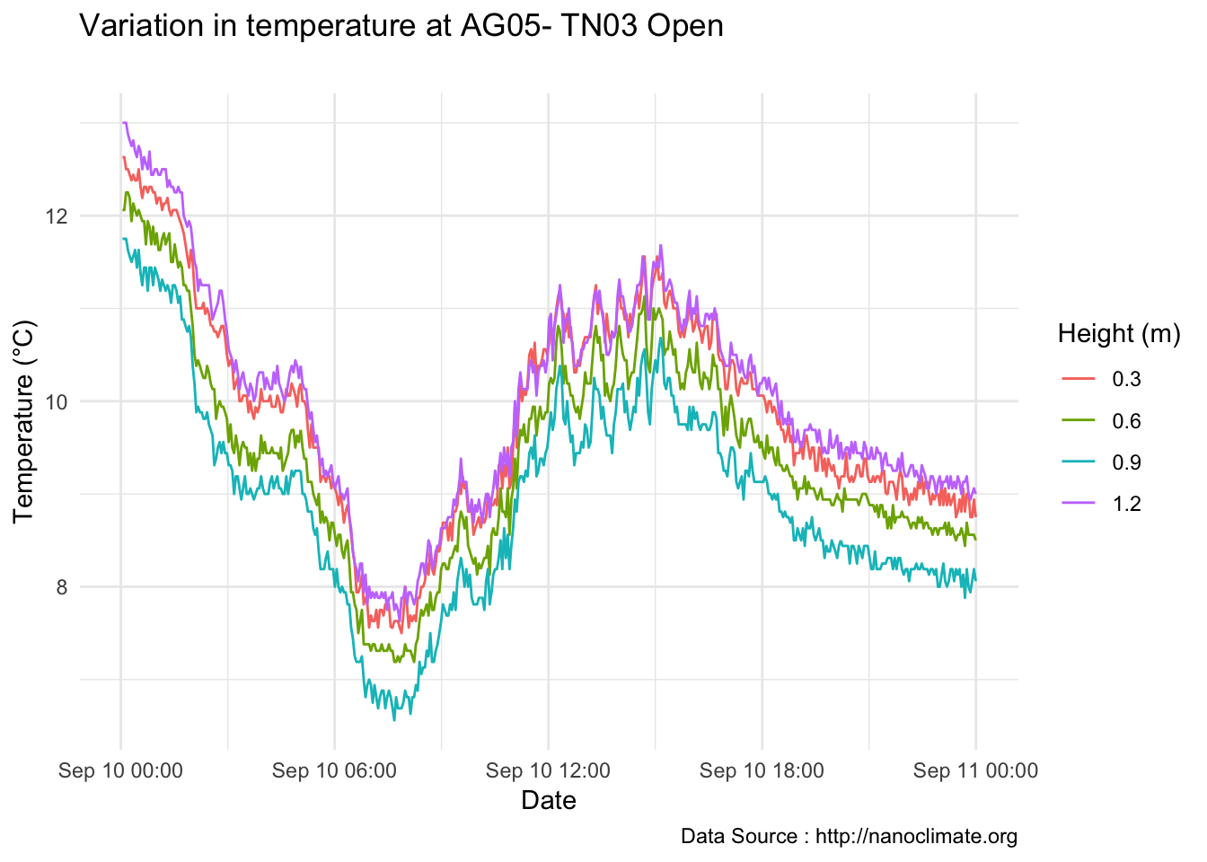
AM16
Narada falls, expect it to be much cooler as its a bog where the CN is and others are little above.
TN01
mclim_AM16_TN01_2018<- read.csv('./data/DATALOG-AM16-TN01.CSV')
names(mclim_AM16_TN01_2018) <- c('time','nodeid','temp','batt')
mclim_AM16_TN01_2018$time <- as.POSIXct(mclim_AM16_TN01_2018$time, "%Y/%m/%d %H:%M:%S")

#Add hour month and day
## 11-05-2018
mclim_AM16_TN01_2018$hr <- hour(mclim_AM16_TN01_2018$time)
mclim_AM16_TN01_2018$minute<- minute(mclim_AM16_TN01_2018$time)
mclim_AM16_TN01_2018$day <- day(mclim_AM16_TN01_2018$time)
mclim_AM16_TN01_2018$month<- month(mclim_AM16_TN01_2018$time)

#Roughly one feet apart
mclim_AM16_TN01_2018$height <- 0

mclim_AM16_TN01_2018[mclim_AM16_TN01_2018$nodeid=='28D216779104027E' ,]$height <- 0.6
mclim_AM16_TN01_2018[mclim_AM16_TN01_2018$nodeid=='28BC8B77910802B8' ,]$height <- 1.2
mclim_AM16_TN01_2018[mclim_AM16_TN01_2018$nodeid=='28B50A7791040265' ,]$height <- 0.3
mclim_AM16_TN01_2018[mclim_AM16_TN01_2018$nodeid=='28B18877910802BC' ,]$height <- 0.9

## Day plot , Representive day
mclim_AM16_TN01_2018 %>% filter(month(time) %in% '9') %>%
ggplot( aes(time,temp,color = factor(height))) + geom_line() + theme_minimal() +
ggtitle("Variation in temperature at AM16- TN01 Closed")  + xlab("Date") +
  ylab("Temperature (°C)") + labs(colour = "Height(m)",
subtitle="9/17/2018",caption="Data Source : http://nanoclimate.org") 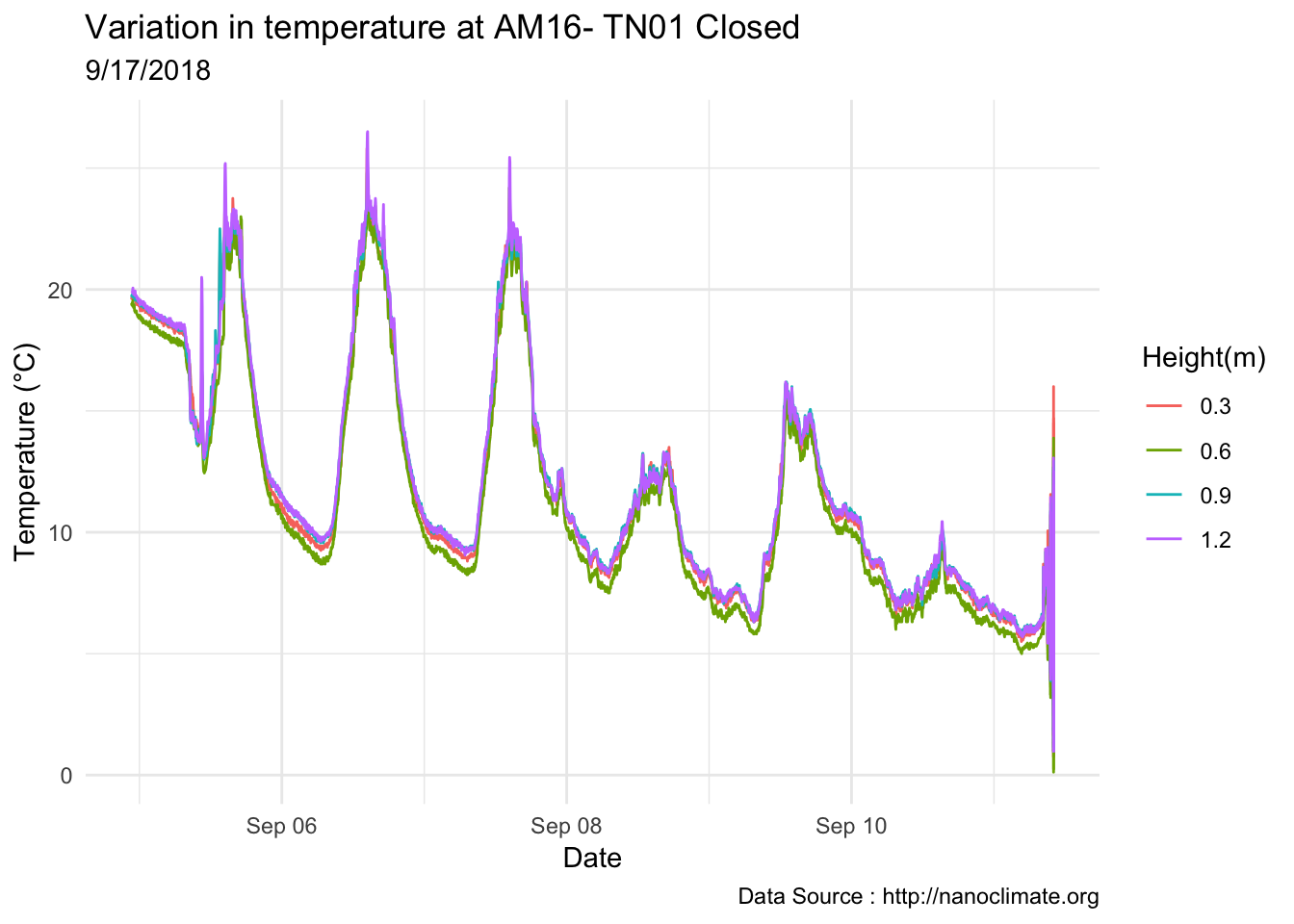
mclim_AM16_TN02_2018<- read.csv('./data/DATALOG-AM16-TN02.CSV')
names(mclim_AM16_TN02_2018) <- c('time','nodeid','temp','batt')
mclim_AM16_TN02_2018$time <- as.POSIXct(mclim_AM16_TN02_2018$time, "%Y/%m/%d %H:%M:%S")

#Add hour month and day
## 11-05-2018
mclim_AM16_TN02_2018$hr <- hour(mclim_AM16_TN02_2018$time)
mclim_AM16_TN02_2018$minute<- minute(mclim_AM16_TN02_2018$time)
mclim_AM16_TN02_2018$day <- day(mclim_AM16_TN02_2018$time)
mclim_AM16_TN02_2018$month<- month(mclim_AM16_TN02_2018$time)

#Roughly one feet apart
mclim_AM16_TN02_2018$height <- 0

mclim_AM16_TN02_2018[mclim_AM16_TN02_2018$nodeid=='28439C77910802C3' ,]$height <- 0.6
mclim_AM16_TN02_2018[mclim_AM16_TN02_2018$nodeid=='28F4B977910902AF' ,]$height <- 1.2
mclim_AM16_TN02_2018[mclim_AM16_TN02_2018$nodeid=='28D9657791100272' ,]$height <- 0.3
mclim_AM16_TN02_2018[mclim_AM16_TN02_2018$nodeid=='28C928779106026A' ,]$height <- 0.9

## Day plot , Representive day
mclim_AM16_TN02_2018 %>% filter(month(time) %in% '9') %>%
ggplot( aes(time,temp,color = factor(height))) + geom_line() + theme_minimal() +
ggtitle("Variation in temperature at AM16- TN02 Closed")  + xlab("Date") +
  ylab("Temperature (°C)") + labs(colour = "Height(m)",
subtitle="9/17/2018",caption="Data Source : http://nanoclimate.org") 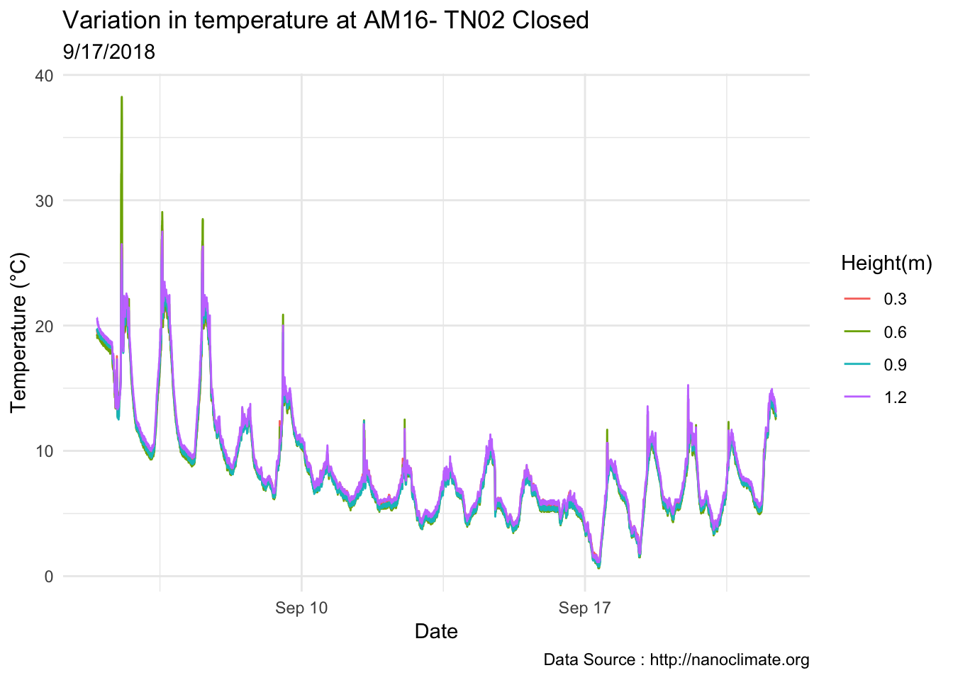
Need to fix the hour
mclim_AM16_TN03_2018<- read.csv('./data/DATALOG-AM16-TN03.CSV')
names(mclim_AM16_TN03_2018) <- c('time','nodeid','temp','batt')
mclim_AM16_TN03_2018$time <- as.POSIXct(mclim_AM16_TN03_2018$time, "%Y/%m/%d %H:%M:%S")

#Add hour month and day
## 11-05-2018
mclim_AM16_TN03_2018$hr <- hour(mclim_AM16_TN03_2018$time)
mclim_AM16_TN03_2018$minute<- minute(mclim_AM16_TN03_2018$time)
mclim_AM16_TN03_2018$day <- day(mclim_AM16_TN03_2018$time)
mclim_AM16_TN03_2018$month<- month(mclim_AM16_TN03_2018$time)

#Roughly one feet apart
mclim_AM16_TN03_2018$height <- 0

mclim_AM16_TN03_2018[mclim_AM16_TN03_2018$nodeid=='28A64677910302C1' ,]$height <- 0.6
mclim_AM16_TN03_2018[mclim_AM16_TN03_2018$nodeid=='28542677910A027E' ,]$height <- 1.2
mclim_AM16_TN03_2018[mclim_AM16_TN03_2018$nodeid=='28EE7977910802DD' ,]$height <- 0.3
mclim_AM16_TN03_2018[mclim_AM16_TN03_2018$nodeid=='283D867791080289' ,]$height <- 0.9

## Day plot , Representive day
mclim_AM16_TN03_2018 %>% filter(month(time) %in% '9' & height !=0) %>%
ggplot( aes(time,temp,color = factor(height))) + geom_line() + theme_minimal() +
ggtitle("Variation in temperature at AM16- TN03 Open")  + xlab("Date") +
  ylab("Temperature (°C)") + labs(colour = "Height(m)",
subtitle="9/17/2018",caption="Data Source : http://nanoclimate.org") 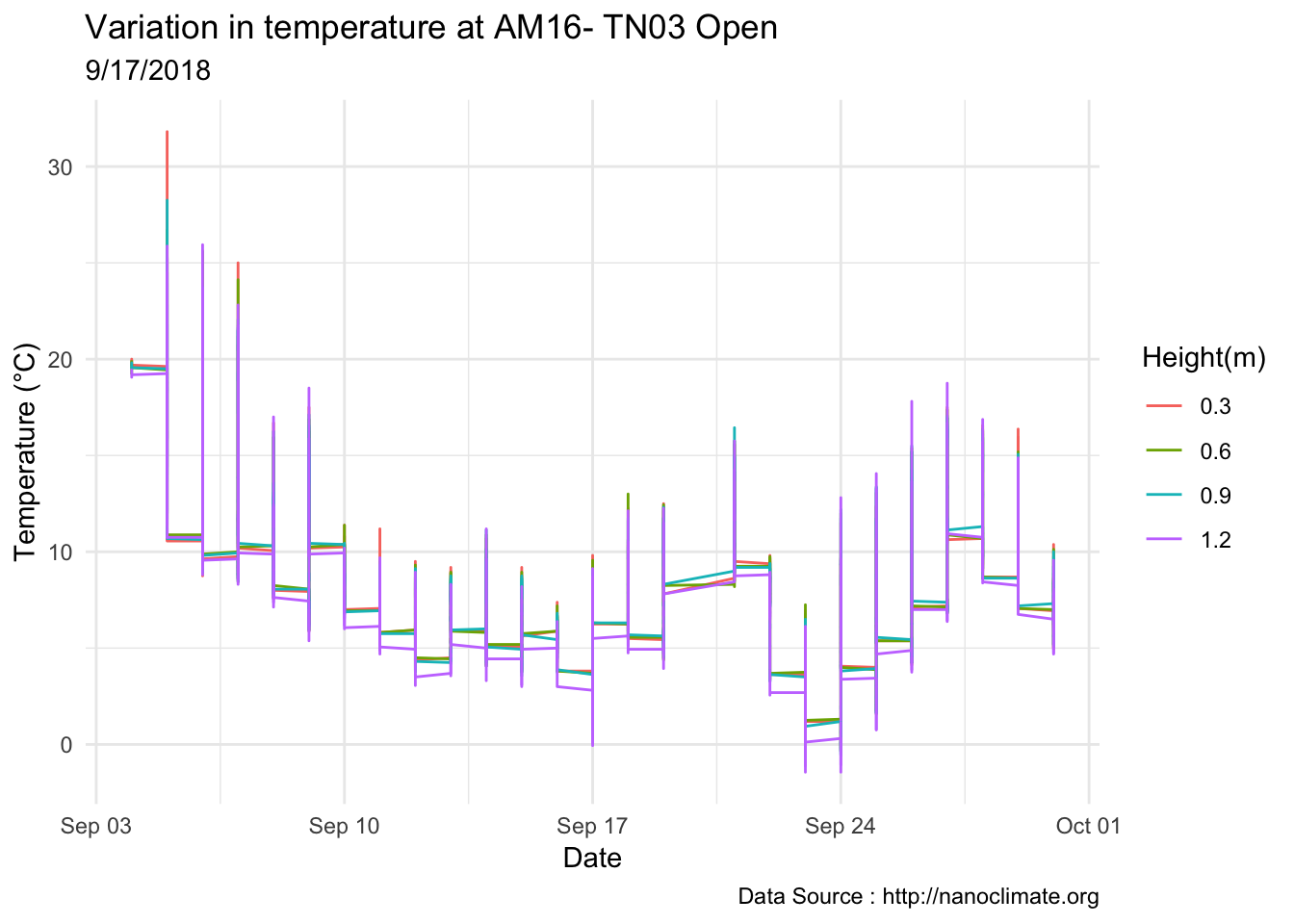
To do CN01 for AM16 which is on the bog.
TO04 - expect it to be cold but stull warmer than the rest
mclim_TO04_TN01_2018<- read.csv('./data/DATALOG-TO04-TN01.CSV')
names(mclim_TO04_TN01_2018) <- c('time','nodeid','temp','batt')
mclim_TO04_TN01_2018$time <- as.POSIXct(mclim_TO04_TN01_2018$time, "%Y/%m/%d %H:%M:%S")
#Add hour month and day
## 11-05-2018
mclim_TO04_TN01_2018$hr <- hour(mclim_TO04_TN01_2018$time)
mclim_TO04_TN01_2018$minute<- minute(mclim_TO04_TN01_2018$time)
mclim_TO04_TN01_2018$day <- day(mclim_TO04_TN01_2018$time)
mclim_TO04_TN01_2018$month<- month(mclim_TO04_TN01_2018$time)
#Roughly one feet apart
mclim_TO04_TN01_2018$height <- 0
mclim_TO04_TN01_2018[mclim_TO04_TN01_2018$nodeid=='2883A377910802B7' ,]$height <- 0.6
mclim_TO04_TN01_2018[mclim_TO04_TN01_2018$nodeid=='28B14477910F02D1' ,]$height <- 1.2
mclim_TO04_TN01_2018[mclim_TO04_TN01_2018$nodeid=='28783877910402B7' ,]$height <- 0.3
mclim_TO04_TN01_2018[mclim_TO04_TN01_2018$nodeid=='286919779106027F' ,]$height <- 0.9
## Day plot , Representive day
mclim_TO04_TN01_2018 %>% filter(month(time) %in% '9' & temp != -127) %>%
ggplot( aes(time,temp,color = factor(height))) + geom_line() + theme_minimal() +
ggtitle("Variation in temperature at TO04- TN01 Closed") + xlab("Date") +
ylab("Temperature (°C)") + labs(colour = "Height(m)",
subtitle="9/17/2018",caption="Data Source : http://nanoclimate.org") 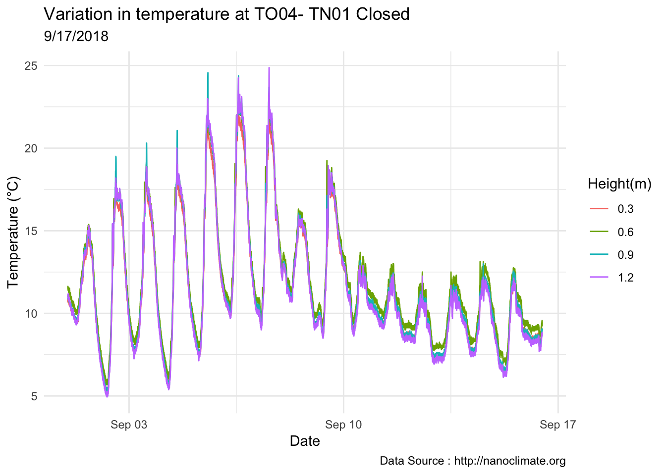
mclim_TO04_TN02_2018<- read.csv('./data/DATALOG-TO04-TN02.CSV')
names(mclim_TO04_TN02_2018) <- c('time','nodeid','temp','batt')
mclim_TO04_TN02_2018$time <- as.POSIXct(mclim_TO04_TN02_2018$time, "%Y/%m/%d %H:%M:%S")
#Add hour month and day
## 11-05-2018
mclim_TO04_TN02_2018$hr <- hour(mclim_TO04_TN02_2018$time)
mclim_TO04_TN02_2018$minute<- minute(mclim_TO04_TN02_2018$time)
mclim_TO04_TN02_2018$day <- day(mclim_TO04_TN02_2018$time)
mclim_TO04_TN02_2018$month<- month(mclim_TO04_TN02_2018$time)
#Roughly one feet apart
mclim_TO04_TN02_2018$height <- 0
mclim_TO04_TN02_2018[mclim_TO04_TN02_2018$nodeid=='28A13C7791130278' ,]$height <- 0.6
mclim_TO04_TN02_2018[mclim_TO04_TN02_2018$nodeid=='2893977791080277' ,]$height <- 1.2
mclim_TO04_TN02_2018[mclim_TO04_TN02_2018$nodeid=='28414B77910F02CC' ,]$height <- 0.3
mclim_TO04_TN02_2018[mclim_TO04_TN02_2018$nodeid=='28F94277910F0299' ,]$height <- 0.9
## Day plot , Representive day
mclim_TO04_TN02_2018 %>% filter(month(time) %in% '9' & temp != -127) %>%
ggplot( aes(time,temp,color = factor(height))) + geom_line() + theme_minimal() +
ggtitle("Variation in temperature at TO04- TN02 Open") + xlab("Date") +
ylab("Temperature (°C)") + labs(colour = "Height(m)",
subtitle="9/17/2018",caption="Data Source : http://nanoclimate.org") 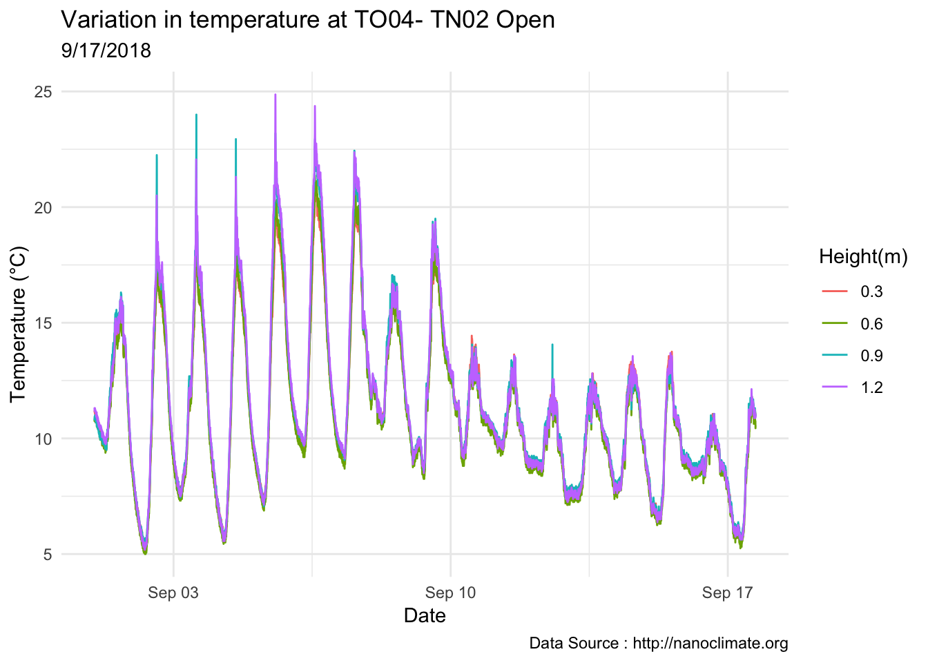
mclim_TO04_TN03_2018<- read.csv('./data/DATALOG-TO04-TN03.CSV')
names(mclim_TO04_TN03_2018) <- c('time','nodeid','temp','batt')
mclim_TO04_TN03_2018$time <- as.POSIXct(mclim_TO04_TN03_2018$time, "%Y/%m/%d %H:%M:%S")
#Add hour month and day
## 11-05-2018
mclim_TO04_TN03_2018$hr <- hour(mclim_TO04_TN03_2018$time)
mclim_TO04_TN03_2018$minute<- minute(mclim_TO04_TN03_2018$time)
mclim_TO04_TN03_2018$day <- day(mclim_TO04_TN03_2018$time)
mclim_TO04_TN03_2018$month<- month(mclim_TO04_TN03_2018$time)
#Roughly one feet apart
mclim_TO04_TN03_2018$height <- 0
mclim_TO04_TN03_2018[mclim_TO04_TN03_2018$nodeid=='28CC077791040287' ,]$height <- 0.6
mclim_TO04_TN03_2018[mclim_TO04_TN03_2018$nodeid=='288EEB77910902EE' ,]$height <- 1.2
mclim_TO04_TN03_2018[mclim_TO04_TN03_2018$nodeid=='28D7C67791090242' ,]$height <- 0.3
mclim_TO04_TN03_2018[mclim_TO04_TN03_2018$nodeid=='286EDA779109028E' ,]$height <- 0.9
## Day plot , Representive day
mclim_TO04_TN03_2018 %>% filter(month(time) %in% '9' & temp != -127) %>%
ggplot( aes(time,temp,color = factor(height))) + geom_line() + theme_minimal() +
ggtitle("Variation in temperature at TO04- TN03 Closed") + xlab("Date") +
ylab("Temperature (°C)") + labs(colour = "Height(m)",
subtitle="9/17/2018",caption="Data Source : http://nanoclimate.org") 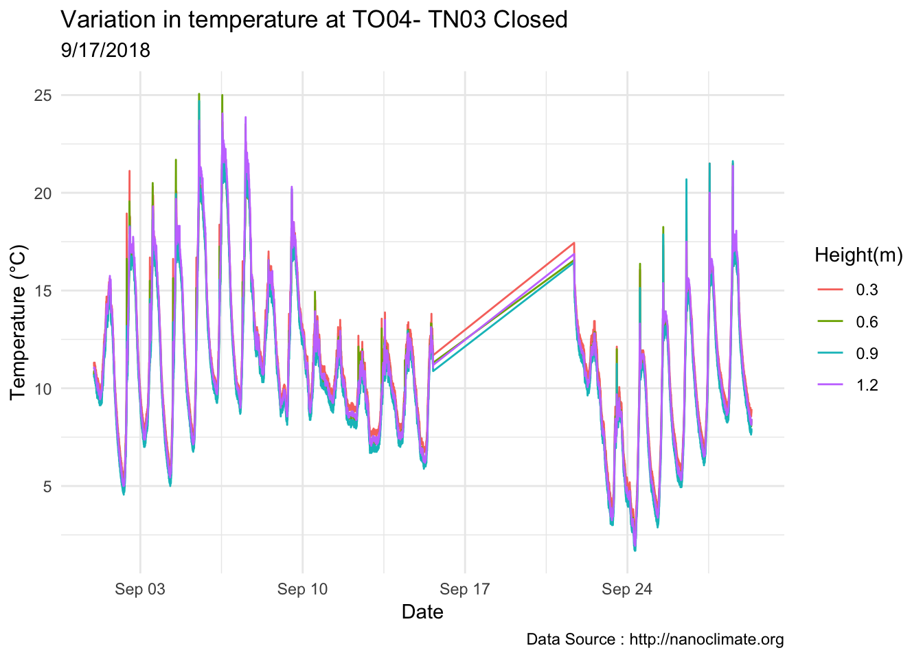
8.30 1-17-2019
ae10_TN01 <- mclim_AE10_TN01_2018 %>%
filter ( month %in% c(9) & height == 0.9) %>%
filter( day > 4 & day < 16) %>%
group_by(month,day,hr) %>%
add_count(wt=3) %>%
summarise(m1= mean(temp)) %>%
group_by(day,hr) %>% as.data.frame()
ae10_TN01$site <- 'AE10_TN01'
ag05_TN01 <- mclim_AG05_TN01_2018 %>%
filter (month %in% c(9) & height == 1.2) %>%
filter( day > 4 & day < 16) %>%
group_by(month,day,hr) %>%
add_count(wt=3) %>%
summarise(m1= mean(temp)) %>%
group_by(day,hr) %>% as.data.frame()
ag05_TN01$site <- 'AG05_TN01'
am16_TN01 <- mclim_AM16_TN01_2018 %>%
filter (month %in% c(9) & height == 1.2) %>%
filter( day > 4 & day < 16) %>%
group_by(month,day,hr) %>%
add_count(wt=3) %>%
summarise(m1= mean(temp)) %>%
group_by(day,hr) %>% as.data.frame()
am16_TN01$site <- 'AM16_TN01'
TO04_TN01 <- mclim_TO04_TN01_2018 %>%
filter (month %in% c(9) & height == 1.2 & temp != -127) %>%
filter( day > 4 & day < 16) %>%
group_by(month,day,hr) %>%
add_count(wt=3) %>%
summarise(m1= mean(temp)) %>%
group_by(day,hr) %>% as.data.frame()
TO04_TN01$site <- 'TO04_TN01'
combined_across_MM <- rbind(ae10_TN01,
ag05_TN01,
am16_TN01,
TO04_TN01,
Paradise_5to15,
Sunrise_5to15)
combined_across_MM %>% filter (month %in% c(9) ) %>%
filter( day %in% c(5,6,7,8,9,10,11,12,13,14) ) %>%
ggplot() +
geom_line(aes(hr,m1,color = site),se=F)+
facet_grid(. ~ day, scales = "free") +
scale_color_manual("Site(m)",values=c("AE10_TN01"=1,"AG05_TN01"=2,"AM16_TN01"=3,"TO04_TN01"=4,"Paradise_1645"=5,"Sunrise_2097"=6)) +
theme_classic() + ggtitle("Diel variation in Temperature at different sites in comparison to micromet") + xlab("Hour") +
ylab("Temperature (°C)") + labs(colour = "Hour",
subtitle="1 hr resolution",caption="Data Source : http://www.nanoclimate.org") 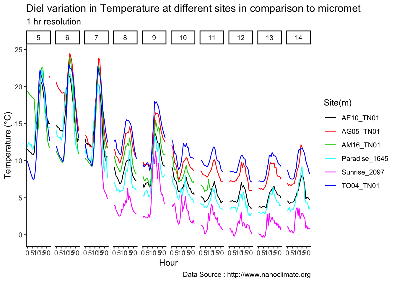
Battery voltages
ae10_TN01_batt <- mclim_AE10_TN01_2018 %>%
filter ( month %in% c(9) & height == 0.9) %>%
filter( day > 4 & day < 16) %>%
group_by(month,day,hr) %>%
add_count(wt=3) %>%
summarise(m1= mean(batt)) %>%
group_by(day,hr) %>% as.data.frame()
ae10_TN01_batt$site <- 'AE10_TN01'
ag05_TN01_batt <- mclim_AG05_TN01_2018 %>%
filter (month %in% c(9) & height == 1.2) %>%
filter( day > 4 & day < 16) %>%
group_by(month,day,hr) %>%
add_count(wt=3) %>%
summarise(m1= mean(batt)) %>%
group_by(day,hr) %>% as.data.frame()
ag05_TN01_batt$site <- 'AG05_TN01'
am16_TN01_batt <- mclim_AM16_TN01_2018 %>%
filter (month %in% c(9) & height == 1.2) %>%
filter( day > 4 & day < 16) %>%
group_by(month,day,hr) %>%
add_count(wt=3) %>%
summarise(m1= mean(batt)) %>%
group_by(day,hr) %>% as.data.frame()
am16_TN01_batt$site <- 'AM16_TN01'
TO04_TN01_batt <- mclim_TO04_TN01_2018 %>%
filter (month %in% c(9) & height == 1.2 ) %>%
filter( day > 4 & day < 16) %>%
group_by(month,day,hr) %>%
add_count(wt=3) %>%
summarise(m1= mean(batt)) %>%
group_by(day,hr) %>% as.data.frame()
TO04_TN01_batt$site <- 'TO04_TN01'
combined_batt_across_MM <- rbind(ae10_TN01_batt,
ag05_TN01_batt,
am16_TN01_batt,
TO04_TN01_batt)
combined_batt_across_MM %>% filter (month %in% c(9) ) %>%
filter( day %in% c(5,6,7,8,9,10,11,12,13,14) ) %>%
ggplot() +
geom_line(aes(hr,m1,color = site),se=F)+
facet_grid(. ~ day, scales = "free") +
scale_color_manual("Site(m)",values=c("AE10_TN01"=1,"AG05_TN01"=2,"AM16_TN01"=3,"TO04_TN01"=4,"Paradise_1645"=5,"Sunrise_2097"=6)) +
theme_classic() + ggtitle("Diel variation in batt at different sMM sites") + xlab("Hour") +
ylab("Temperature (°C)") + labs(colour = "Hour",
subtitle="1 hr resolution",caption="Data Source : http://www.nanoclimate.org") 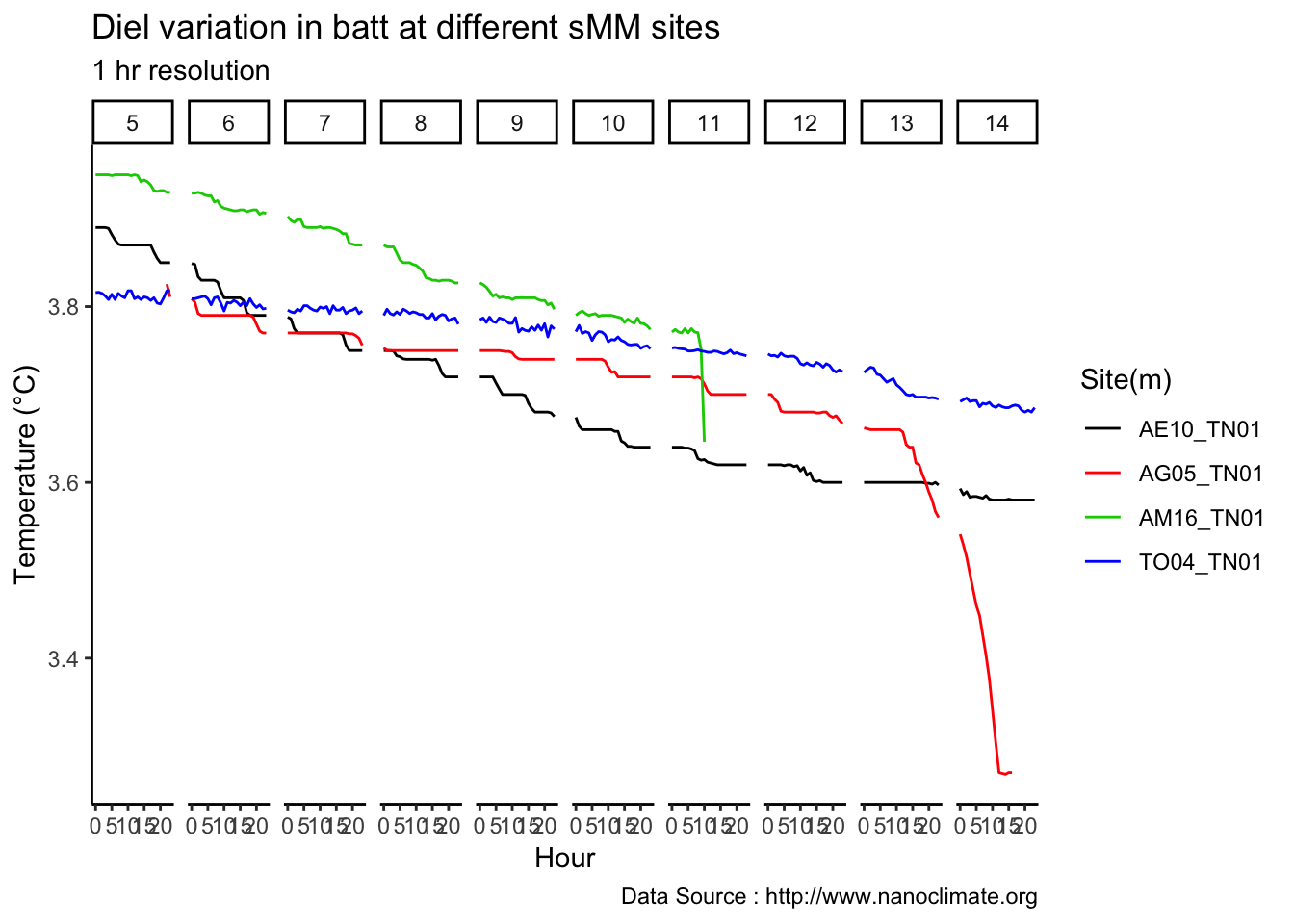
Difference between the heights
ggplot(data=mclim_AM16_TN01_2018, aes(x=as.factor(height), y=temp)) +
geom_boxplot(aes(fill=as.factor(height))) +
ylab("Temperature") + xlab("Height") +ggtitle("AM16 -Narada Temp Boxplot") +
stat_summary(fun.y=mean, geom="point", shape=5, size=4) +
theme_minimal()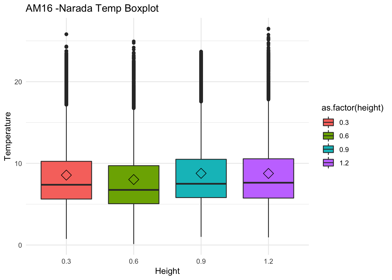
mclim_AE10_TN01_2018 %>% filter(temp != -127) %>%
ggplot(aes(x=as.factor(height), y=temp)) +
geom_boxplot(aes(fill=as.factor(height))) +
ylab("Temperature") + xlab("Height") +ggtitle("AE10 -Reflection Temp Boxplot") +
stat_summary(fun.y=mean, geom="point", shape=5, size=4) +
theme_minimal()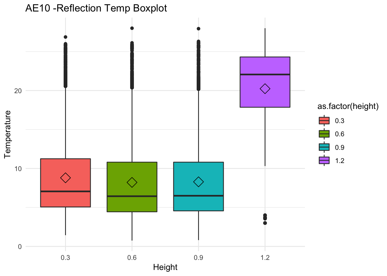
mclim_AG05_TN01_2018 %>% filter(temp != -127) %>%
ggplot(aes(x=as.factor(height), y=temp)) +
geom_boxplot(aes(fill=as.factor(height))) +
ylab("Temperature") + xlab("Height") +ggtitle("AG05 -Longmire Temp Boxplot") +
stat_summary(fun.y=mean, geom="point", shape=5, size=4) +
theme_minimal()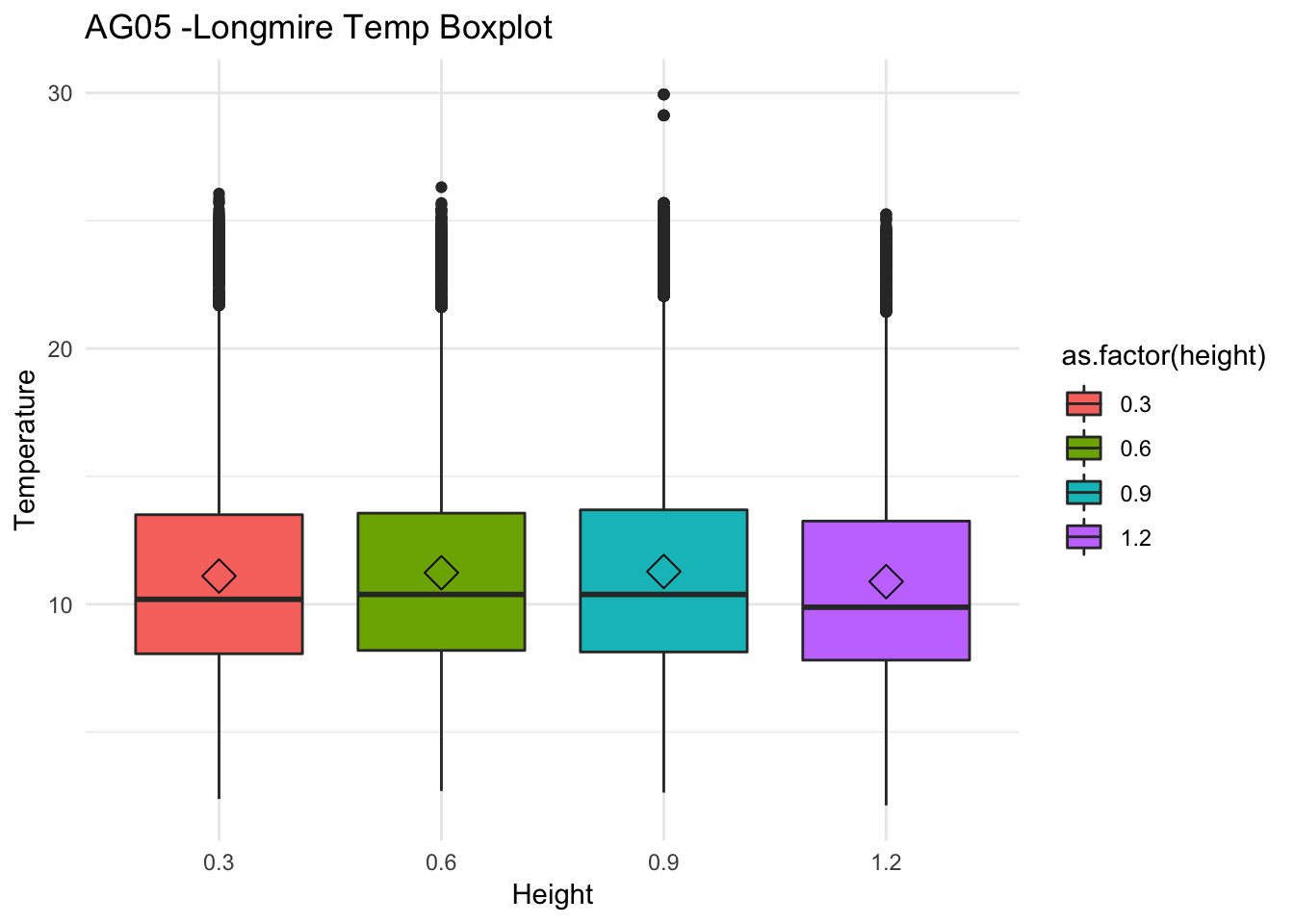
mclim_TO04_TN01_2018 %>% filter(temp != -127) %>%
ggplot(aes(x=as.factor(height), y=temp)) +
geom_boxplot(aes(fill=as.factor(height))) +
ylab("Temperature") + xlab("Height") +ggtitle("TO04 -Devils Temp Boxplot") +
stat_summary(fun.y=mean, geom="point", shape=5, size=4) +
theme_minimal()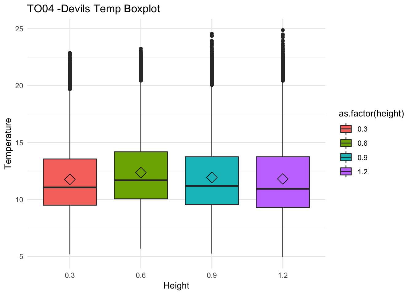
Open vs Closed - Expect to see higher temperatures ad more variability
AE10 - TN01 - Open AM16 - TN01 - Closed AG05 - TN01 - Closed TO04 - TN01 - Closed
Looking at the above plots AE10 is warmer than the rest.
0.3 must be more turbulent than the rest, is it ?
mclim_TO04_TN01_2018 %>% filter(temp != -127) %>%
dplyr::group_by(height) %>%
dplyr::summarise(meant = mean(temp), cft = sd(temp)) %>%
ggplot(aes(x=as.factor(height), y=cft)) +
geom_boxplot(aes(fill=as.factor(height))) +
ylab("Temperature") + xlab("Height") +ggtitle("TO04 -Devils SD Temp Boxplot") +
stat_summary(fun.y=mean, geom="point", shape=5, size=4) +
theme_minimal()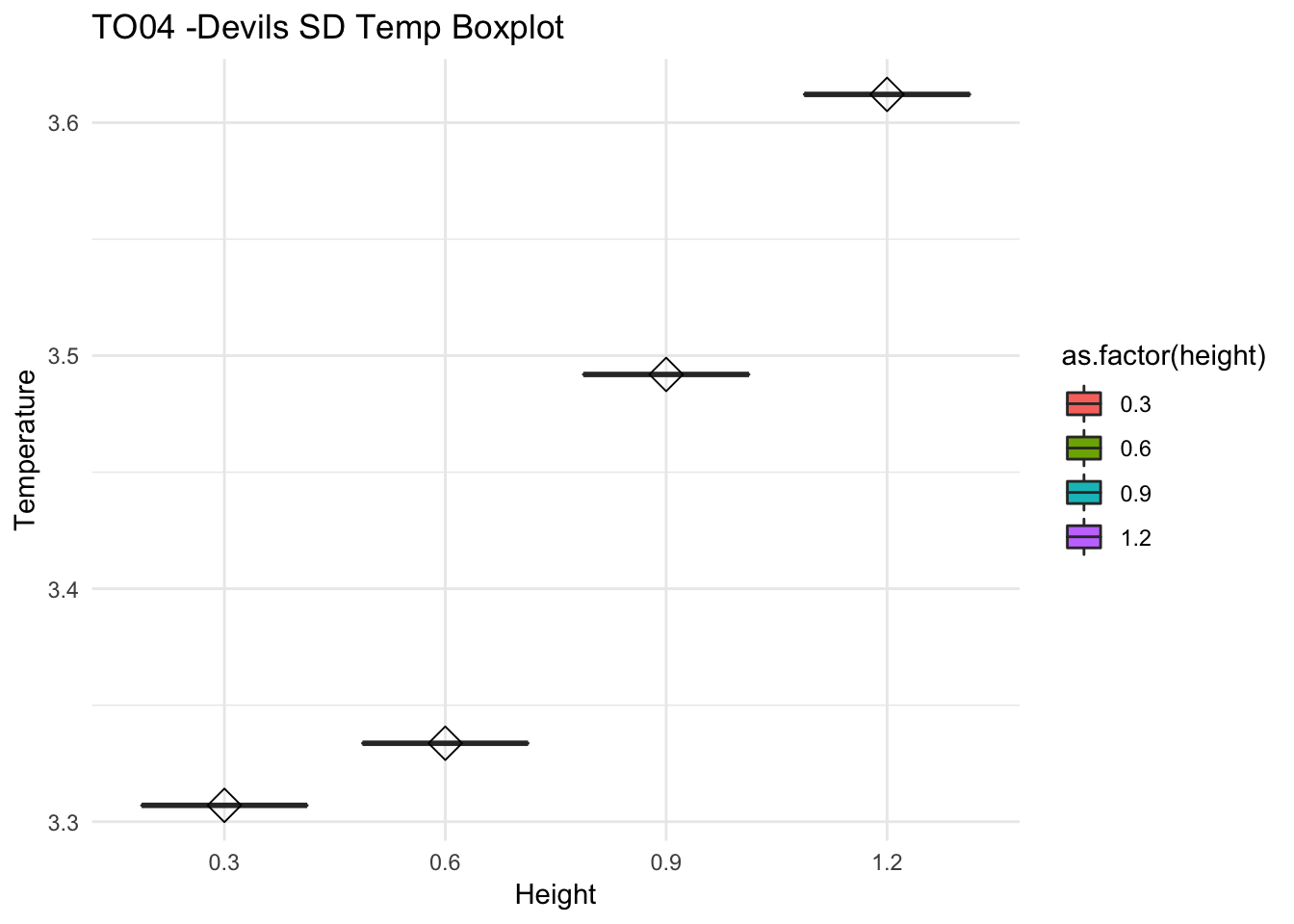
Looks like SD is the highest for 1.2 height, is it true for all of them ?
mclim_AG05_TN01_2018 %>% filter(temp != -127) %>%
dplyr::group_by(height) %>%
dplyr::summarise(meant = mean(temp), cft = sd(temp)) %>%
ggplot(aes(x=as.factor(height), y=cft)) +
geom_boxplot(aes(fill=as.factor(height))) +
ylab("Temperature") + xlab("Height") +ggtitle("AG05 -Longmire SD Temp Boxplot") +
stat_summary(fun.y=mean, geom="point", shape=5, size=4) +
theme_minimal()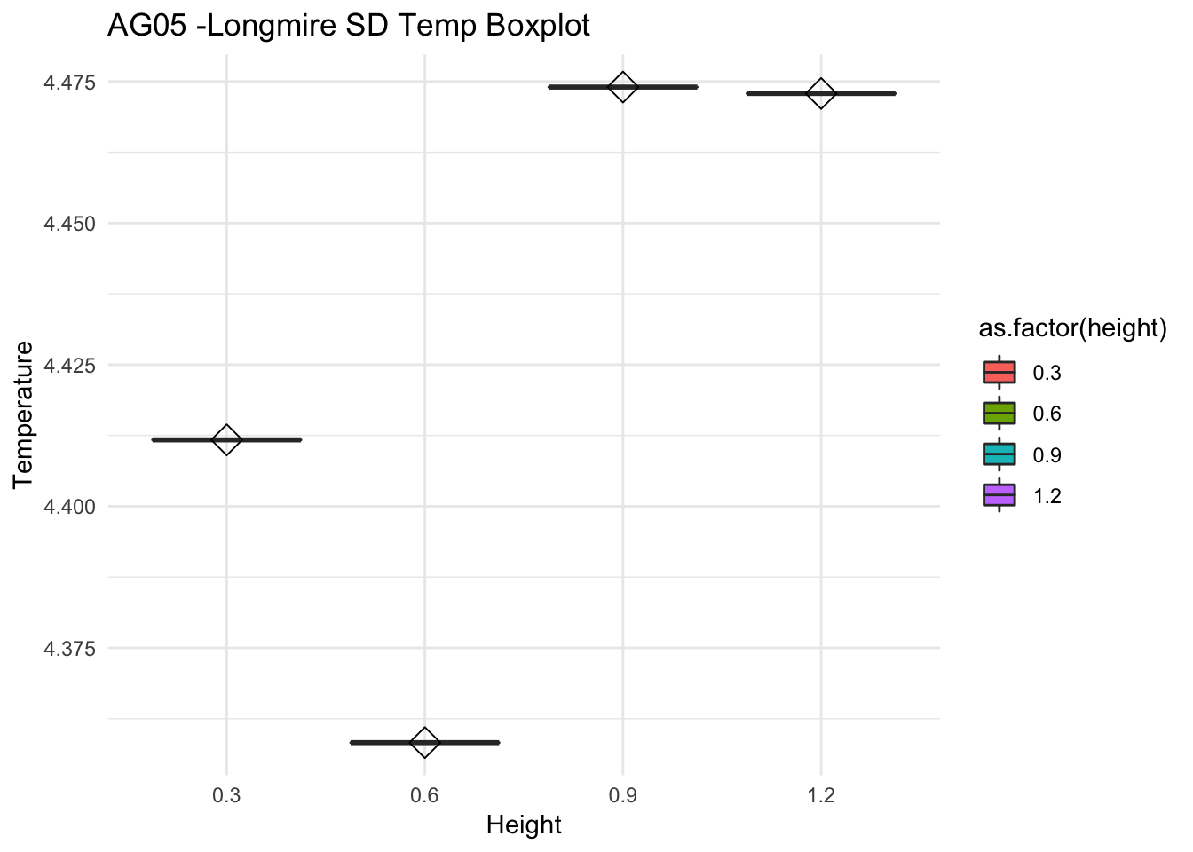
mclim_AM16_TN01_2018 %>% filter(temp != -127) %>%
dplyr::group_by(height) %>%
dplyr::summarise(meant = mean(temp), cft = sd(temp)) %>%
ggplot(aes(x=as.factor(height), y=cft)) +
geom_boxplot(aes(fill=as.factor(height))) +
ylab("Temperature") + xlab("Height") +ggtitle("AM16 -Narada falls SD Temp Boxplot") +
stat_summary(fun.y=mean, geom="point", shape=5, size=4) +
theme_minimal()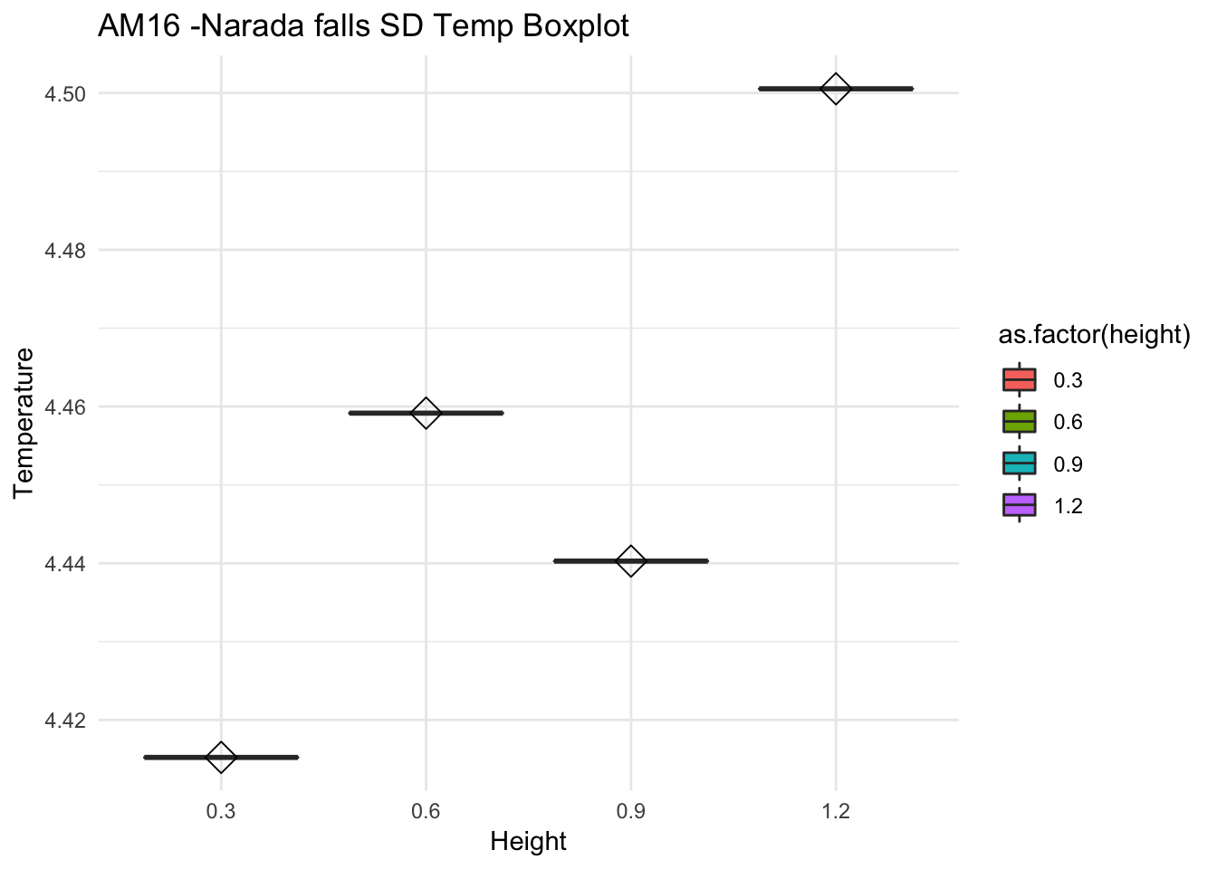
Falls in place for AM16, lets check fpr AE10
mclim_AE10_TN01_2018 %>% filter(temp != -127) %>%
dplyr::group_by(height) %>%
dplyr::summarise(meant = mean(temp), cft = sd(temp)) %>%
ggplot(aes(x=as.factor(height), y=cft)) +
geom_boxplot(aes(fill=as.factor(height))) +
ylab("Temperature") + xlab("Height") +ggtitle("AE10 -Reflection falls SD Temp Boxplot") +
stat_summary(fun.y=mean, geom="point", shape=5, size=4) +
theme_minimal()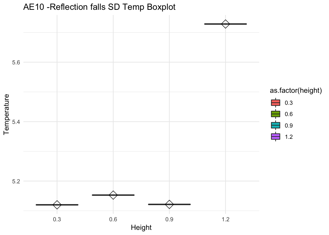 ## 1-18-2019
Longmire hourly data
MtRainier_coopsnowsep_longmire %>%
filter(year== 2018) %>%
ggplot() +
geom_line(aes(Day,as.numeric(Min_Temperature),col='1')) +
geom_line(aes(Day,as.numeric(Max_Temperature),col='2')) +
geom_line(data=MtRainier_coopsnowsep_skatecreek,aes(Day,as.numeric(Min_Temperature),col='3')) +
geom_line(data=MtRainier_coopsnowsep_skatecreek,aes(Day,as.numeric(Max_Temperature),col='4')) +
geom_line(data=MtRainier_coopsnowsep_Paradise,aes(Day,as.numeric(Min_Temperature),col='5')) +
geom_line(data=MtRainier_coopsnowsep_Paradise,aes(Day,as.numeric(Max_Temperature),col='6')) +
theme_classic() + labs(x="Date", y="Temperature(°C) ",subtitle="Coop/Snotel - Mt Rainier- Minimum/Max Recorded every day (2018) ", caption="Data Source : utah state climate center") +
geom_hline(aes(yintercept=9),colour="black", linetype="dashed") +
scale_colour_manual(name = 'Heights(m)',
values =c('1','2','3','4','5','6'), labels = c('841(Longmire)-Min ','841(Longmire)-Max ','1149(Skatecreek)-Min','1149(Skatecreek)-Max',"1654(Paradise)-Min","1654
(Paradise)-Max"))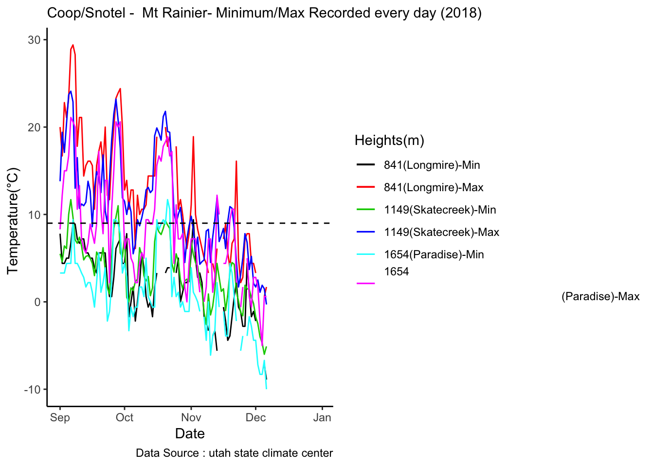
# head(MtRainier_coopsnowsep_longmire)
#
# daily_longmire <- data.frame()
# # R function
# #get hourly temperatures
# dtf = function(x, output) {
# # x is the row of type Character
# # access element in first column
# date = x[1]
# # min
# min = as.numeric(x[3])
#
# # max
# max = as.numeric(x[4])
#
# # day
# day = x[5]
#
# # month
# month = x[6]
#
# # year
# year = x[7]
#
# for (hr in 1:24)
# {
# dayrecords <- TrenchR::diurnal_temp_variation_sine(Tmn=min,Tmx=max,Hr=hr)
# print(paste(date,dayrecords,hr,min,max,day,month,year,sep = ','))
# daily_longmire <- rbind(daily_longmire, dayrecords)
# }
#
#
# }
#
# MtRainier_coopsnowsep_longmire_ss <- MtRainier_coopsnowsep_longmire %>% dplyr::filter(month==9 & day > 0 & day < 25) %>% as.data.frame()
#
# MtRainier_coopsnowsep_longmire_ss$Min_Temperature <- as.numeric(MtRainier_coopsnowsep_longmire_ss$Min_Temperature)
#
# MtRainier_coopsnowsep_longmire_ss$Max_Temperature <- as.numeric(MtRainier_coopsnowsep_longmire_ss$Max_Temperature)
#
# df <- apply(MtRainier_coopsnowsep_longmire_ss, 1, dtf)Prepare Longmire hourly
longmire_hrly <- read_csv('./data/longmire_hourly')## Parsed with column specification:
## cols(
## date = col_date(format = ""),
## m1 = col_double(),
## hr = col_double(),
## min = col_double(),
## max = col_double(),
## day = col_double(),
## month = col_double(),
## year = col_double()
## ) longmire_hrly_5to15 <- longmire_hrly %>% filter (month %in% c(9)) %>%
filter( day > 4 & day < 16) %>%
group_by(month,day,hr) %>%
add_count(wt=3) %>%
summarise(m1= mean(m1)) %>%
group_by(day,hr) %>% as.data.frame()
longmire_hrly_5to15$site <- 'Longmire_841' ae10_TN01 <- mclim_AE10_TN01_2018 %>%
filter ( month %in% c(9) & height == 0.9) %>%
filter( day > 4 & day < 16) %>%
group_by(month,day,hr) %>%
add_count(wt=3) %>%
dplyr::summarise(m1= mean(temp)) %>%
group_by(day,hr) %>% as.data.frame()
ae10_TN01$site <- 'AE10_TN01_1450'
ag05_TN01 <- mclim_AG05_TN01_2018 %>%
filter (month %in% c(9) & height == 1.2) %>%
filter( day > 4 & day < 16) %>%
group_by(month,day,hr) %>%
add_count(wt=3) %>%
dplyr::summarise(m1= mean(temp)) %>%
group_by(day,hr) %>% as.data.frame()
ag05_TN01$site <- 'AG05_TN01_950'
am16_TN01 <- mclim_AM16_TN01_2018 %>%
filter (month %in% c(9) & height == 1.2) %>%
filter( day > 4 & day < 16) %>%
group_by(month,day,hr) %>%
add_count(wt=3) %>%
dplyr::summarise(m1= mean(temp)) %>%
group_by(day,hr) %>% as.data.frame()
am16_TN01$site <- 'AM16_TN01_1200'
TO04_TN01 <- mclim_TO04_TN01_2018 %>%
filter (month %in% c(9) & height == 1.2 & temp != -127) %>%
filter( day > 4 & day < 16) %>%
group_by(month,day,hr) %>%
add_count(wt=3) %>%
dplyr::summarise(m1= mean(temp)) %>%
group_by(day,hr) %>% as.data.frame()
TO04_TN01$site <- 'TO04_TN01_650'
combined_across_MM <- rbind(ae10_TN01,
ag05_TN01,
am16_TN01,
TO04_TN01,longmire_hrly_5to15,
Paradise_5to15,
Sunrise_5to15)
combined_across_MM %>% filter (month %in% c(9) ) %>%
filter( day %in% c(5,6,7,8,9,10,11,12,13,14) ) %>%
ggplot() +
geom_line(aes(hr,m1,color = site),se=F)+
facet_grid(. ~ day, scales = "free") +
scale_color_manual("Site(m)",values=c("AE10_TN01_1450"=1,"AG05_TN01_950"=2,"AM16_TN01_1200"=3,"TO04_TN01_650"=4,"Paradise_1645"=5,"Sunrise_2097"=6,"Longmire_841"=8)) +
theme_classic() + ggtitle("Diel variation in Temperature at different sites in comparison to micromet") + xlab("Hour") +
theme_minimal(base_size=24) +
theme(legend.position = 'bottom',axis.text.x=element_text(angle=90)) +
ylab("Temperature (°C)") + labs(colour = "Hour",
subtitle="1 hr resolution",caption="Data Source : http://www.nanoclimate.org") 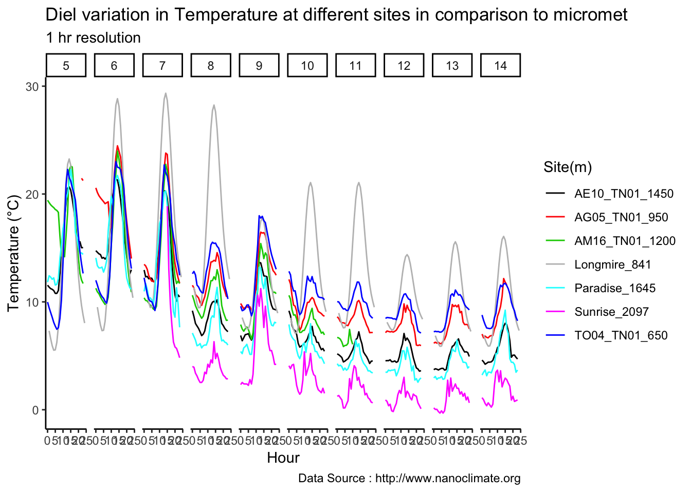
ggsave("mm_comparedtocaorse.png",dpi=300, dev='png', height=8, width=14, units="in") Check the CV
mclim_TO04_TN01_2018 %>% filter(temp != -127) %>%
dplyr::group_by(height) %>%
dplyr::summarise(meant = mean(temp), cft = sd(temp)) %>%
ggplot(aes(x=as.factor(height), y=cft/meant)) +
geom_boxplot(aes(fill=as.factor(height))) +
ylab("Temperature") + xlab("Height") +ggtitle("TO04 -Devils CV Temp Boxplot") +
stat_summary(fun.y=mean, geom="point", shape=5, size=4) +
theme_minimal()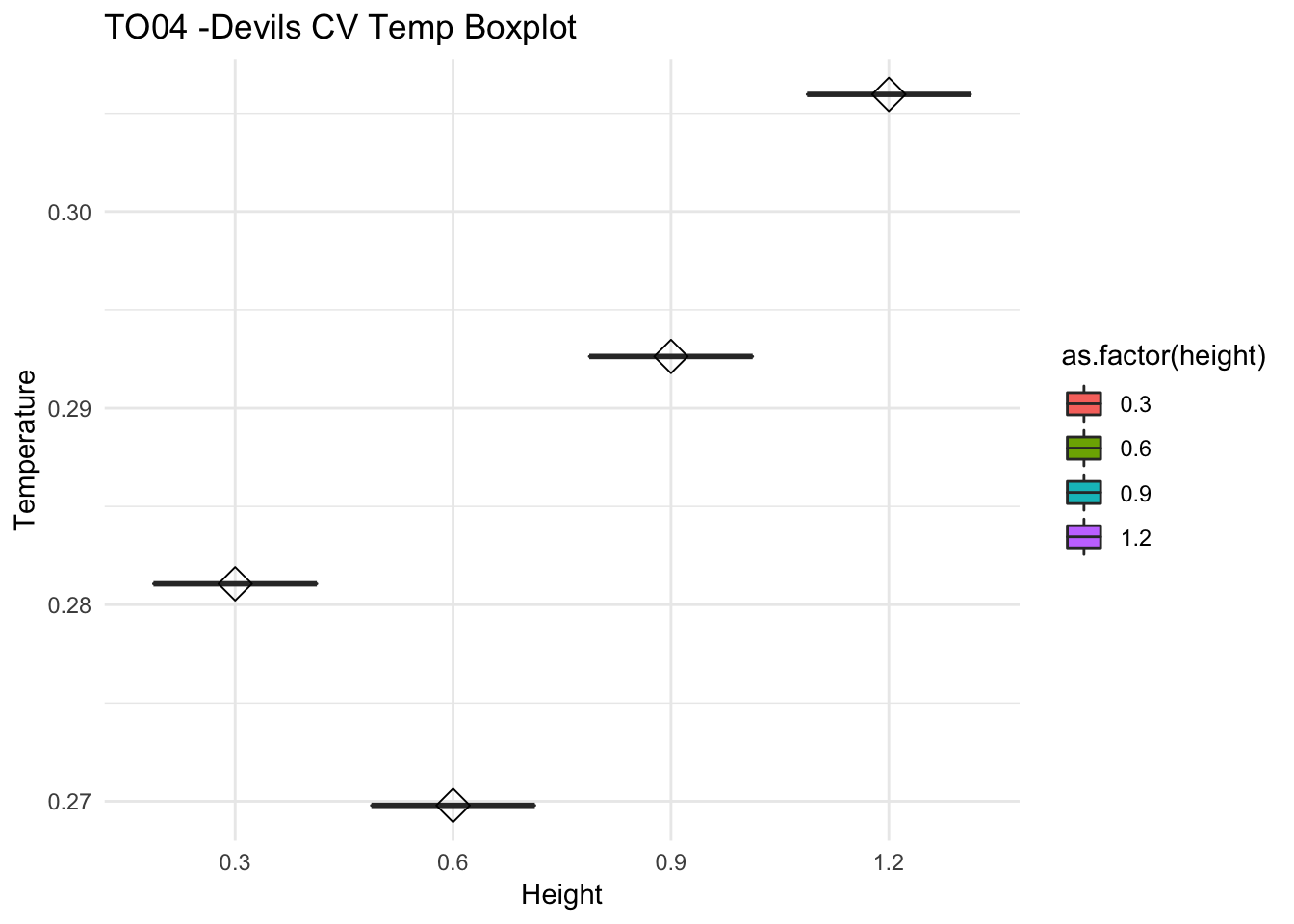
mclim_AE10_TN01_2018 %>% filter(temp != -127) %>%
dplyr::group_by(height) %>%
dplyr::summarise(meant = mean(temp), cft = sd(temp)) %>%
ggplot(aes(x=as.factor(height), y=cft/meant)) +
geom_boxplot(aes(fill=as.factor(height))) +
ylab("Temperature") + xlab("Height") +ggtitle("AE16 -Ref lakes CV Temp Boxplot") +
stat_summary(fun.y=mean, geom="point", shape=5, size=4) +
theme_minimal()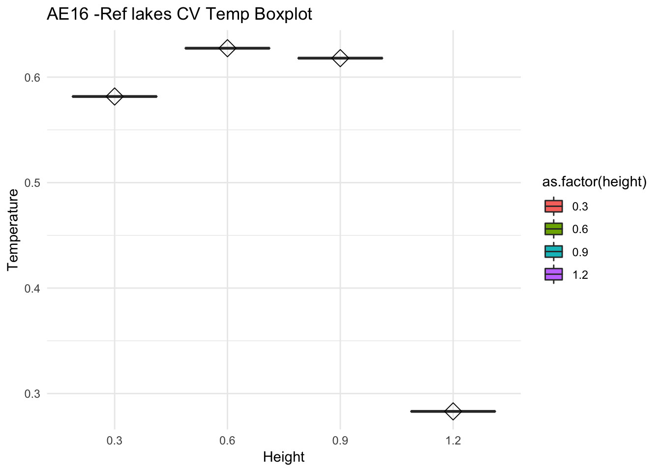
mclim_AM16_TN01_2018 %>% filter(temp != -127) %>%
dplyr::group_by(height) %>%
dplyr::summarise(meant = mean(temp), cft = sd(temp)) %>%
ggplot(aes(x=as.factor(height), y=cft/meant)) +
geom_boxplot(aes(fill=as.factor(height))) +
ylab("Temperature") + xlab("Height") +ggtitle("AM16 -Narada CV Temp Boxplot") +
stat_summary(fun.y=mean, geom="point", shape=5, size=4) +
theme_minimal()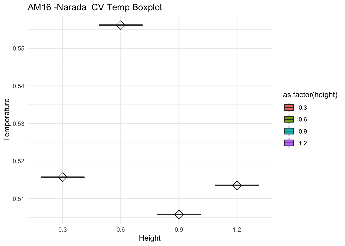
mclim_AG05_TN01_2018 %>% filter(temp != -127) %>%
dplyr::group_by(height) %>%
dplyr::summarise(meant = mean(temp), cft = sd(temp)) %>%
ggplot(aes(x=as.factor(height), y=cft/meant)) +
geom_boxplot(aes(fill=as.factor(height))) +
ylab("Temperature") + xlab("Height") +ggtitle("AG05 -Longmire CV Temp Boxplot") +
stat_summary(fun.y=mean, geom="point", shape=5, size=4) +
theme_minimal()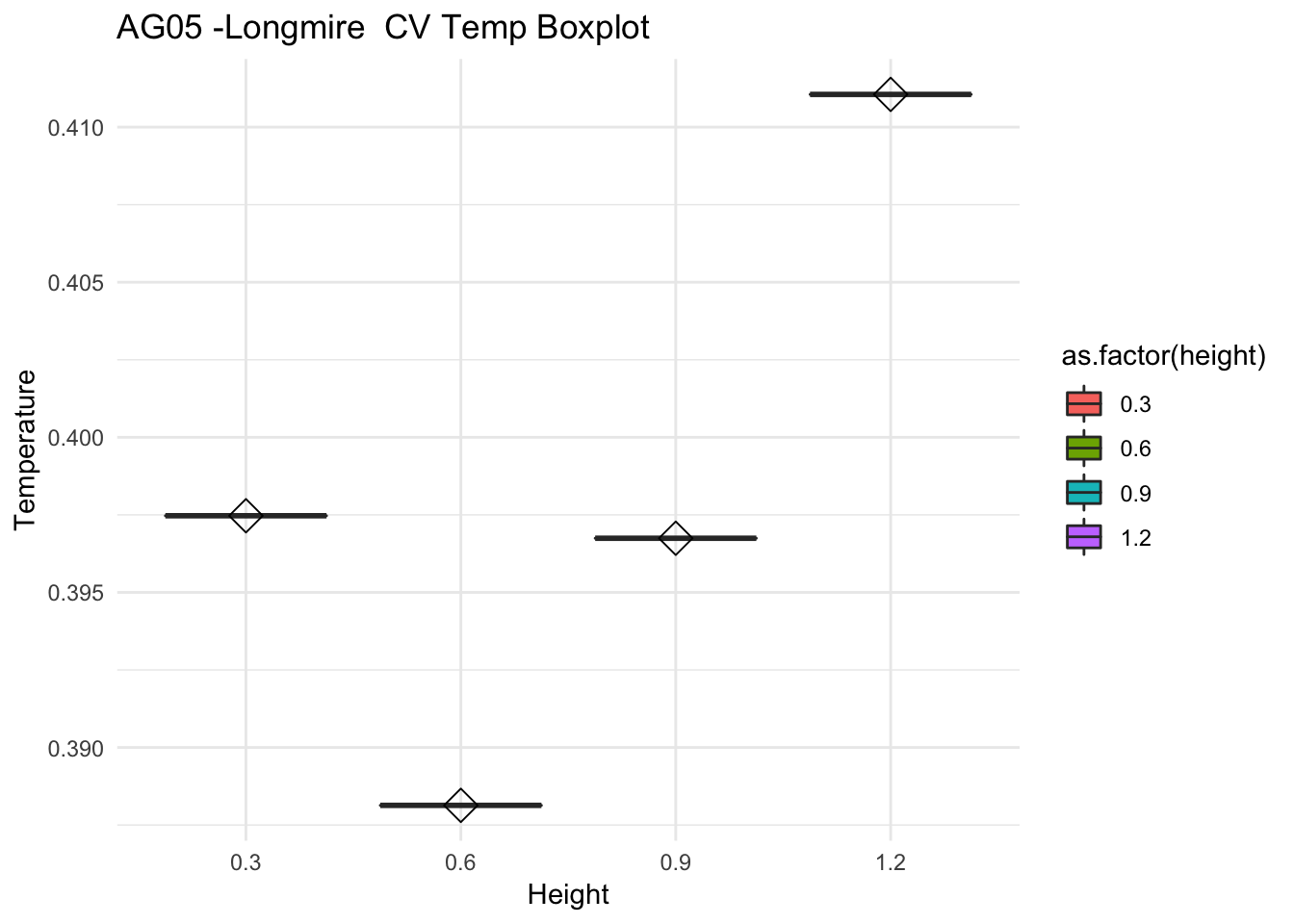
8.31 1-24-2019
Verify Part 2
ae10_TN01_2 <- mclim_AE10_TN01_2018 %>% filter(temp != -127) %>%
filter ( month %in% c(9) & height == 0.9) %>%
filter( day > 14 & day < 30) %>%
group_by(month,day,hr) %>%
add_count(wt=3) %>%
summarise(m1= mean(temp)) %>%
group_by(day,hr) %>% as.data.frame()
ae10_TN01_2$site <- 'AE10_TN01_1450'
ag05_TN02_2 <- mclim_AG05_TN02_2018 %>% filter(temp != -127) %>%
filter (month %in% c(9) & height == 1.2) %>%
filter( day > 14 & day < 30) %>%
group_by(month,day,hr) %>%
add_count(wt=3) %>%
summarise(m1= mean(temp)) %>%
group_by(day,hr) %>% as.data.frame()
ag05_TN02_2$site <- 'AG05_TN02_950'
am16_TN02_2 <- mclim_AM16_TN02_2018 %>% filter(temp != -127) %>%
filter (month %in% c(9) & height == 1.2) %>%
filter( day > 14 & day < 30) %>%
group_by(month,day,hr) %>%
add_count(wt=3) %>%
summarise(m1= mean(temp)) %>%
group_by(day,hr) %>% as.data.frame()
am16_TN02_2$site <- 'AM16_TN02_1200'
TO04_TN03_2 <- mclim_TO04_TN03_2018 %>%
filter (month %in% c(9) & height == 1.2 & temp != -127) %>%
filter( day > 14 & day < 30) %>%
group_by(month,day,hr) %>%
add_count(wt=3) %>%
summarise(m1= mean(temp)) %>%
group_by(day,hr) %>% as.data.frame()
TO04_TN03_2$site <- 'TO04_TN03_650'
longmire_hrly_2 <- longmire_hrly %>% filter (month %in% c(9)) %>%
filter( day > 14 & day < 30) %>%
group_by(month,day,hr) %>%
add_count(wt=3) %>%
summarise(m1= mean(m1)) %>%
group_by(day,hr) %>% as.data.frame()
longmire_hrly_2$site <- 'Longmire_841'
Paradise_2 <- MtRainier_Local_2018 %>% filter (month %in% c(9) ) %>%
filter( day > 14 & day < 30) %>% mutate(m1=(Paradise_5400 - 32) * (5/9)) %>%
group_by(month,day,hr) %>%
dplyr::select(month,day,hr,m1) %>% as.data.frame()
Paradise_2$site <- 'Paradise_1645'
Sunrise_2 <- MtRainier_Local_2018 %>% filter (month %in% c(9) ) %>%
filter( day > 14 & day < 30) %>% mutate(m1=(Sunrise_6880 - 32) * (5/9)) %>%
group_by(month,day,hr) %>%
dplyr::select(month,day,hr,m1) %>% as.data.frame()
Sunrise_2$site <- 'Sunrise_2097'
combined_across_MM_2 <- rbind(ae10_TN01_2,
ag05_TN02_2,
am16_TN02_2,
TO04_TN03_2,
longmire_hrly_2,
Paradise_2,
Sunrise_2)
combined_across_MM_2 %>% filter (month %in% c(9) ) %>%
filter( day %in% c(15,16,17,18,19,20,21,22,23,24,25,26,27,28,29,30) ) %>%
ggplot() +
geom_line(aes(hr,m1,color = site),se=F)+
facet_grid(. ~ day, scales = "free") +
scale_color_manual("Site(m)",values=c("AE10_TN01_1450"=1,"AG05_TN02_950"=2,"AM16_TN02_1200"=3,"TO04_TN03_650"=4,"Paradise_1645"=5,"Sunrise_2097"=6,"Longmire_841"=8)) +
theme_classic() + ggtitle("Diel variation in Temperature at different sites in comparison to micromet") + xlab("Hour") +
ylab("Temperature (°C)") + labs(colour = "Hour",
subtitle="1 hr resolution",caption="Data Source : http://www.nanoclimate.org") 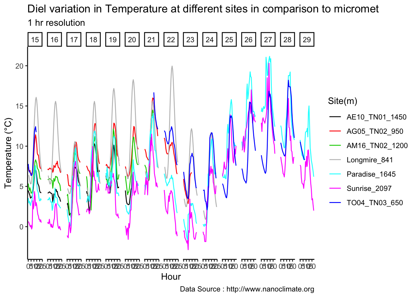
All the dates
ae10_1 <- ae10_TN01
ae10_1$site <- 'AE10_1450'
ag05_1 <- ag05_TN01
ag05_1$site <- 'AG05_950'
am16_1 <- am16_TN01
am16_1$site <- 'AM16_1200'
TO04_1 <- TO04_TN01
TO04_1$site <- 'TO04_650'
Longmire_1 <-longmire_hrly_5to15
Longmire_1$site <- 'Longmire_841'
Paradise_1 <-Paradise_5to15
Paradise_1$site <- 'Paradise_1645'
#Sunrise_1 <-Sunrise_5to15
Sunrise_1 <- Sunrise_5to15
Sunrise_1$site <- 'Sunrise_2097'
ae10_2 <- ae10_TN01_2
ae10_2$site <- 'AE10_1450'
ag05_2 <- ag05_TN02_2
ag05_2$site <- 'AG05_950'
am16_2 <-am16_TN02_2
am16_2$site <- 'AM16_1200'
TO04_2 <- TO04_TN03_2
TO04_2$site <- 'TO04_650'
Longmire_2 <- longmire_hrly_2
Longmire_2$site <- 'Longmire_841'
Paradise_2 <- Paradise_2
Paradise_2$site <- 'Paradise_1645'
Sunrise_2 <- Sunrise_2
Sunrise_2$site <- 'Sunrise_2097'
combined_across_MM_and_PP_Long <- rbind(ae10_1,
ag05_1,
am16_1,
TO04_1,
Longmire_1,
Paradise_1,
Sunrise_1,
ae10_2,
ag05_2,
am16_2,
TO04_2,
Longmire_2,
Paradise_2,
Sunrise_2)
combined_across_MM_and_PP_Long %>% filter (month %in% c(9) ) %>%
ggplot() +
geom_line(aes(hr,m1,color = site),se=F)+
facet_grid(. ~ day, scales = "free") +
scale_color_manual("Site(m)",values=c("AE10_1450"=1,"AG05_950"=2,"AM16_1200"=3,"TO04_650"=4,"Paradise_1645"=5,"Sunrise_2097"=6,"Longmire_841"=8)) +
theme_classic() + ggtitle("Diel variation in Temperature at different sites in comparison to micromet") + xlab("Hour") +
ylab("Temperature (°C)") + labs(colour = "Hour",
subtitle="1 hr resolution",caption="Data Source : http://www.nanoclimate.org") 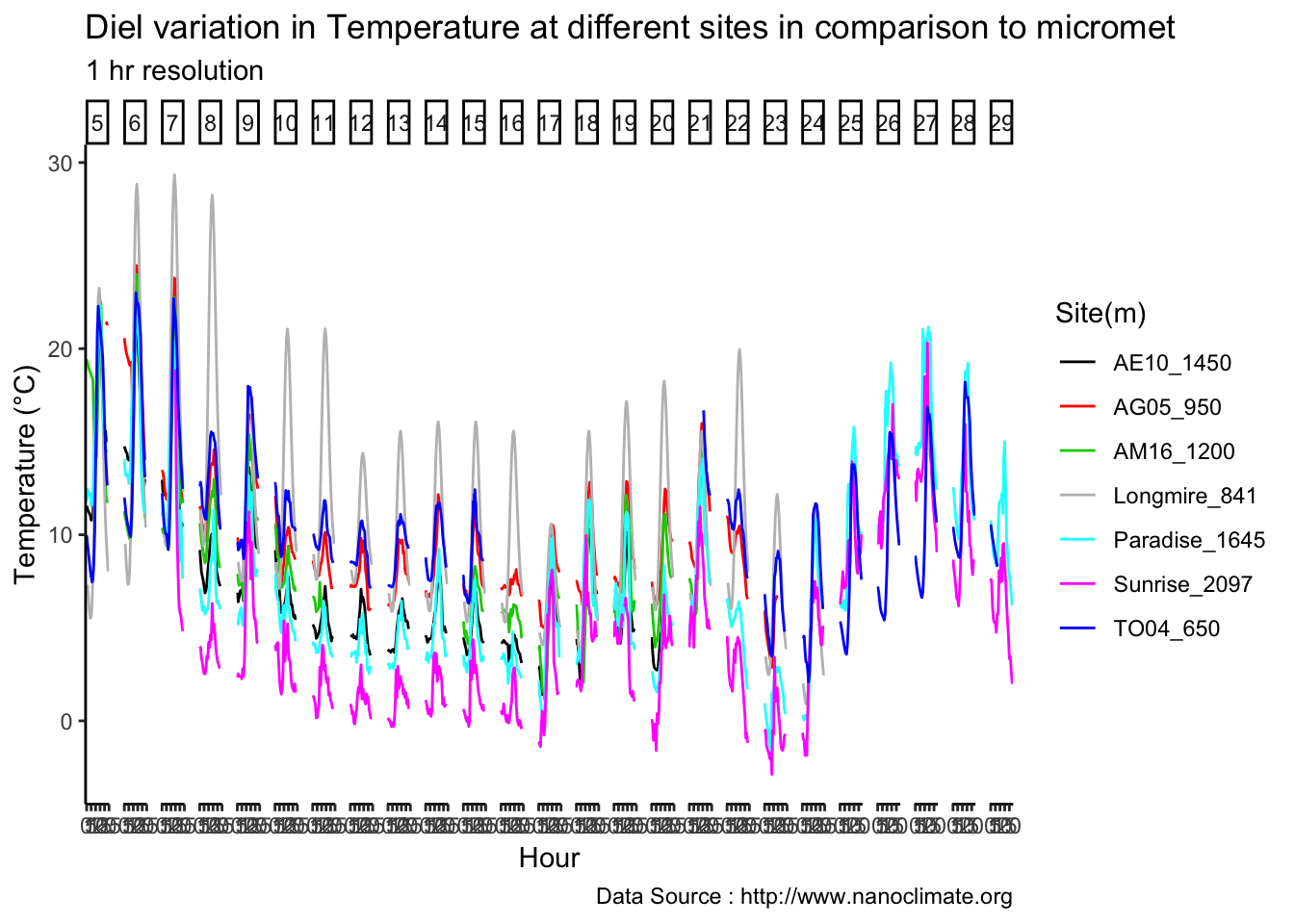
8.32 1-29-2019
Do we see distinct diurnal patterns at differnt height, is it relavsnt to the plants
Get the te,p profile
8.33 2-03-2019
Below canopy you get 1% of sunlight, what does that translate to ?
- compare it with JHRL lux
There is no simple conversion….it depends on the wavelength or color of the light. However, for the SUN, there is an approximate conversion of 0.0079 W/m2 per Lux.(ResearchGate)
AE10_S1_2018<- read.csv('./data/2018/AE10-S1.csv')
colnames(AE10_S1_2018) <- c('#','datetime','Temp','Lux','CoupAttach','HostConn','Stopped','eof')
AE10_S1_2018$timect <- as.POSIXct(AE10_S1_2018$datetime, format="%m/%d/%y %I:%M:%S %p",tz="America/Los_Angeles")
AE10_S1_2018$hr <- hour(AE10_S1_2018$timect)
AE10_S1_2018$minute <- minute(AE10_S1_2018$timect)
AE10_S1_2018$day <- day(AE10_S1_2018$timect)
AE10_S1_2018$month<- month(AE10_S1_2018$timect)
AE10_S1_2018$year<- year(AE10_S1_2018$timect)
AE10_S1_2018 %>%
ggplot() +
geom_point(aes(timect,Temp,col='AE10-S1')) +
geom_line(aes(timect,Temp)) +
theme_classic() + labs(x="Date", y="Temperature(°C) ",subtitle="Air hobo AE10 S1 - Mt Rainie -Recorded every 3 hours (2018) ", caption="Data Source : JHRL") +
geom_hline(aes(yintercept=9),colour="black", linetype="dashed") +
scale_colour_manual(name = 'Heights(m)',
values =c('red','blue','green'), labels = c('1645','2097',"3081"))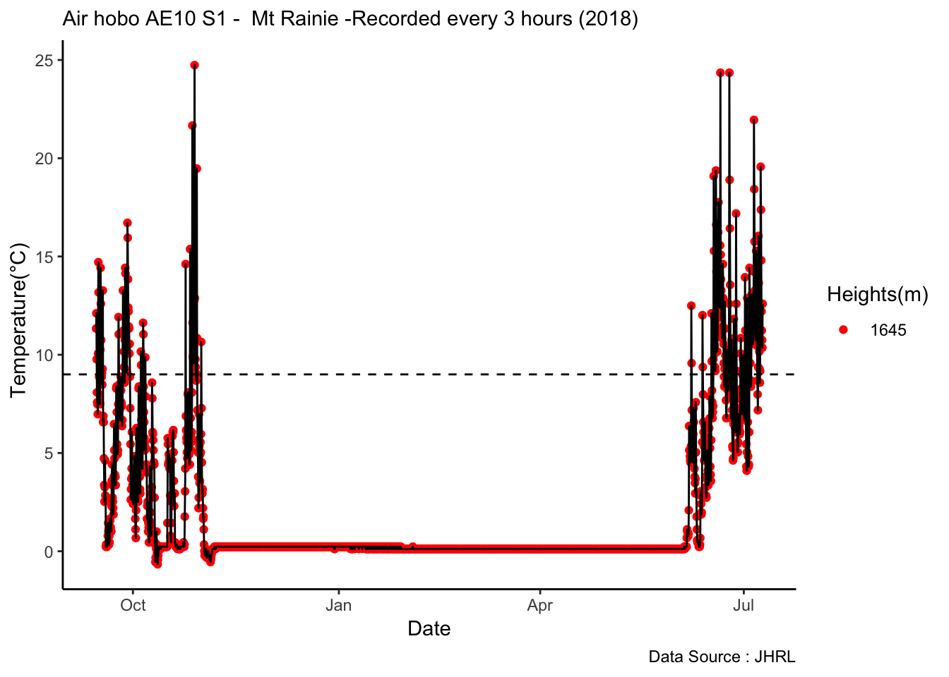
Lets compare temperature of 2017
AE10_S1_2018 %>% filter(year %in% c(2017)) %>%
ggplot() +
geom_point(aes(timect,Temp,col='AE10-S1')) +
geom_line(aes(timect,Temp)) +
theme_classic() + labs(x="Date", y="Temperature(°C) ",subtitle="Air hobo AE10 S1 - Mt Rainie -Recorded every 3 hours (2018) ", caption="Data Source : JHRL") +
geom_hline(aes(yintercept=9),colour="black", linetype="dashed") +
scale_colour_manual(name = 'Heights(m)',
values =c('red','blue','green'), labels = c('1645','2097',"3081"))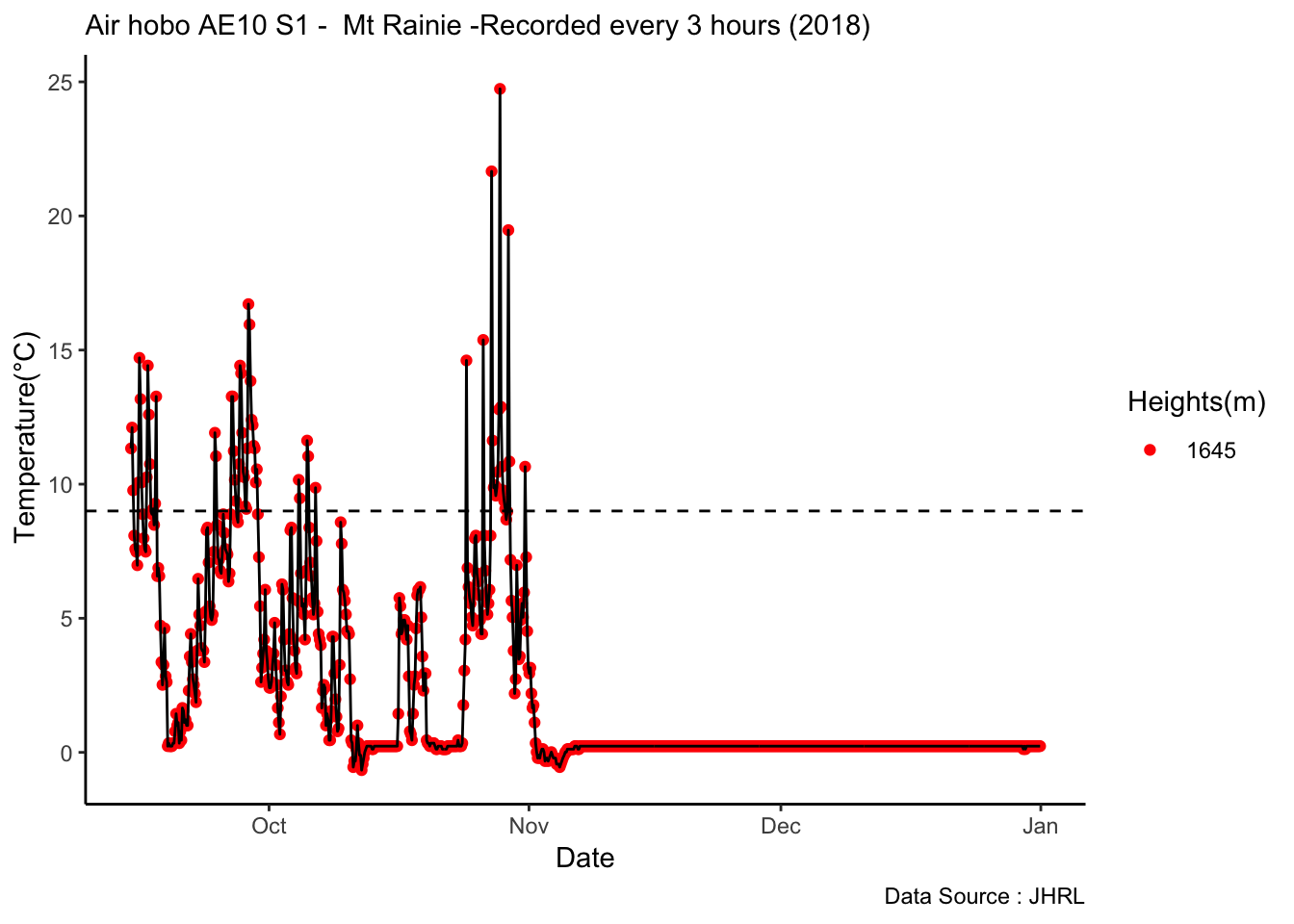
Lot of days where its colder, compare it with air temp for same year at 1.2 , should tell the kind of height relation
AE10_S1_2018 %>% filter(year %in% c(2017) & month %in% c(9,10)) %>%
ggplot() +
# geom_point(aes(timect,Temp,col='AE10-S1')) +
geom_line(aes(timect,Temp,col='S1')) +
geom_line(data=MtRainier_AE10A1_1718[MtRainier_AE10A1_1718$year==2017 & MtRainier_AE10A1_1718$month %in% c(9,10),],aes(timect,Temp,col='M1')) +
# geom_point(data=MtRainier_AE10A1_1718[MtRainier_AE10A1_1718$year==2017 & MtRainier_AE10A1_1718$month %in% c(9,10),],aes(timect,Temp,col='AE10-A1')) +
theme_classic() + labs(x="Date", y="Temperature(°C) ",subtitle="Air hobo AE10 S1 - Mt Rainie -Recorded every 3 hours (2018) ", caption="Data Source : JHRL") +
geom_hline(aes(yintercept=9),colour="black", linetype="dashed") 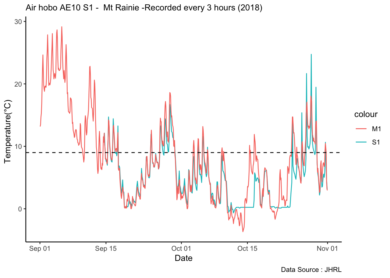
Ground temp looks warmer, lets look for a shorter week
8.34 2-04-2019
AE10_S1_2018 %>% filter(year %in% c(2017) &
month %in% c(9) &
day %in% c(15:25)
) %>%
ggplot() +
# geom_point(aes(timect,Temp,col='AE10-S1')) +
geom_line(aes(hr,Temp,col='S1')) +
geom_line(data=MtRainier_AE10A1_1718[MtRainier_AE10A1_1718$year==2017 & MtRainier_AE10A1_1718$month %in% c(9) &
MtRainier_AE10A1_1718$day %in% c(15:25),],aes(hr,Temp,col='M1')) +
# geom_point(data=MtRainier_AE10A1_1718[MtRainier_AE10A1_1718$year==2017 & MtRainier_AE10A1_1718$month %in% c(9,10),],aes(timect,Temp,col='AE10-A1')) +
facet_grid(. ~ day, scales = "free") +
theme_classic() + labs(x="Date", y="Temperature(°C) ",subtitle="Air hobo AE10 S1 - Mt Rainie -Recorded every 3 hours (2017) ", caption="Data Source : JHRL") +
geom_hline(aes(yintercept=9),colour="black", linetype="dashed") 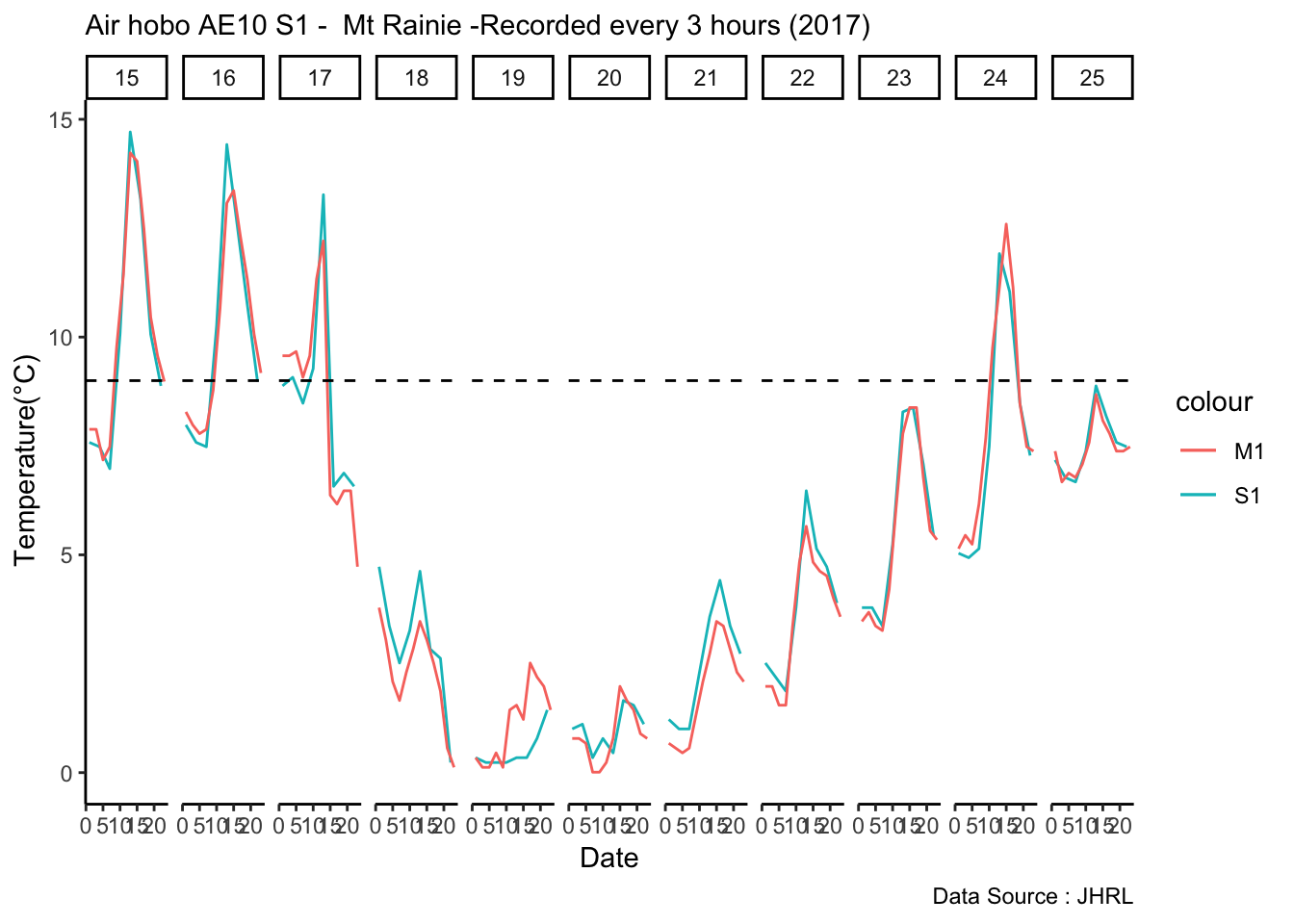
Todo, explain one day of two curves, look at solar radiation for Lux and Paradise The conversion of Lux to W/m^2
https://cumulus.hosiene.co.uk/viewtopic.php?t=3979
AE10_S1_2018 %>% filter(year %in% c(2017) &
month %in% c(9) & day %in% c(15:25)
) %>%
mutate(LuxinWM2 = Lux * 0.0079 ) %>%
ggplot() +
geom_line(aes(hr,LuxinWM2,col='S1')) +
geom_line(data = Paradise_2017[Paradise_2017$month %in% c('09') & Paradise_2017$day %in% c(17:25),], aes(hour,Solar.Pyranometer..W.m2.,col='Paradise') ) +
geom_line(data = Paradise_2017[Paradise_2017$month %in% c('09') & Paradise_2017$day %in% c(17:25),], aes(hour,.05* Solar.Pyranometer..W.m2.,col='Paradise5Pct') ) +
facet_grid(. ~ day, scales = "free") +
# scale_x_datetime(labels=date_format("%H")) +
theme(axis.text.x=element_text(angle=90)) +
theme_classic() + labs(colour = "Site",x="Date", y=" Solar Irradiance(W/m^2) ",subtitle="Ground Lux S1 AE10 compared to Paradise -Recorded every 3 hours (Sept 2017) ", caption="Data Source : JHRL") 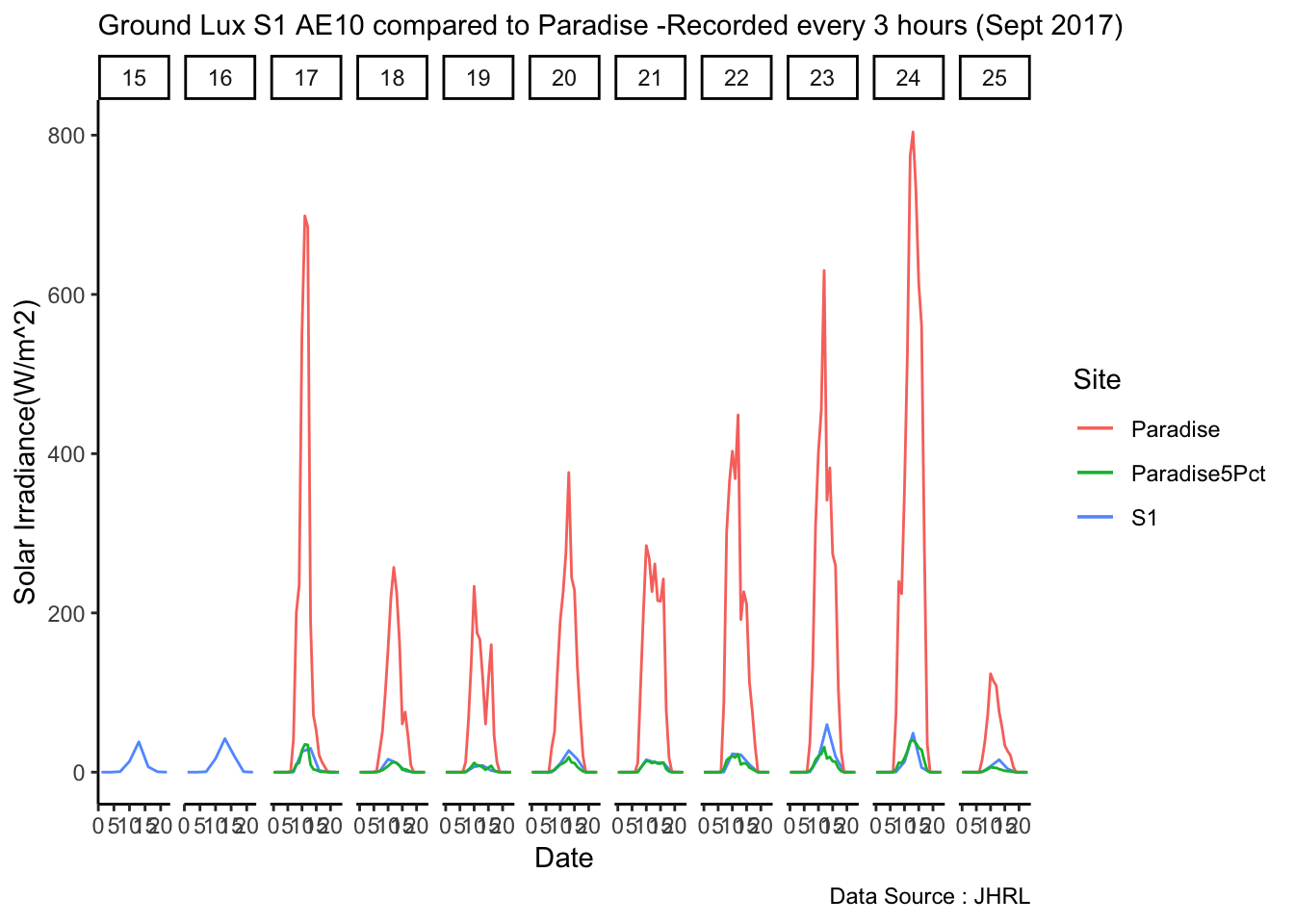
So, ground solar radiation is less than what is above canopy
So, if our scaling is correct, looks like Ground is warmer than on colder days or when its overcast
Lets compare it with Paradise (5400), if clouds are below the elevation, then it should be more warmer (i.e. the AE10 sites)
AE10_S1_2018 %>% filter(year %in% c(2017) &
month %in% c(9) &
day %in% c(15:25)
) %>%
ggplot() +
# geom_point(aes(timect,Temp,col='AE10-S1')) +
geom_line(aes(hr,Temp,col='S1')) +
geom_line(data=MtRainier_AE10A1_1718[MtRainier_AE10A1_1718$year==2017 & MtRainier_AE10A1_1718$month %in% c(9) &
MtRainier_AE10A1_1718$day %in% c(15:25),],aes(hr,Temp,col='M1')) +
geom_line(data=Paradise_5400_2017[Paradise_5400_2017$month %in% c(9) & Paradise_5400_2017$day %in% c(15:25),],aes(hr,weathermetrics::fahrenheit.to.celsius(Temperature..deg.F.),col='Paradise')) +
# geom_point(data=MtRainier_AE10A1_1718[MtRainier_AE10A1_1718$year==2017 & MtRainier_AE10A1_1718$month %in% c(9,10),],aes(timect,Temp,col='AE10-A1')) +
facet_grid(. ~ day, scales = "free") +
theme_classic() + labs(x="Date", y="Temperature(°C) ",subtitle="Air hobo AE10 S1 - Mt Rainier -Recorded every 3 hours (2017) ", caption="Data Source : JHRL") +
geom_hline(aes(yintercept=9),colour="black", linetype="dashed") 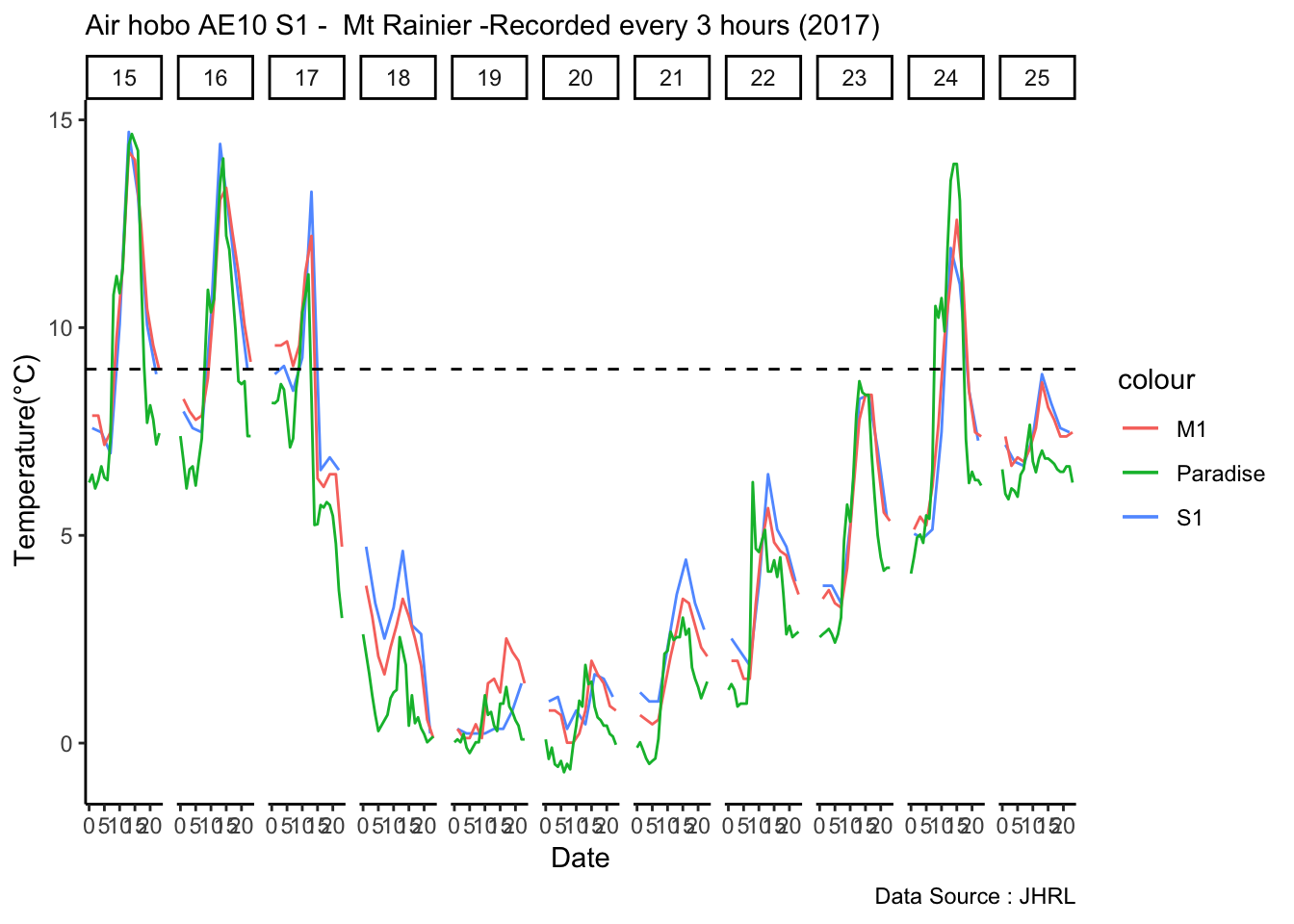
Some days, looks like cold days, the ground is warmer consistently, even much warmer than the air temp for the same day.
Ideal - In the mornings ground is coller than air, till yu reach solar max (11 am), after yu get to max, the ground is much warmer, so the air is less warmer than ground, and it remains like it thru early mornings.
Switching back to year 2019, lets liok at how the Solar radation load looked like
AM16
mclim_AM16_CN01_2018<-read_csv('./data/DATALOG-AM16-CN01.CSV')## Parsed with column specification:
## cols(
## date = col_character(),
## temp1 = col_double(),
## temp2 = col_double(),
## temp3 = col_double(),
## temp4 = col_double(),
## windspeed1 = col_double(),
## windspeed2 = col_double(),
## windspeed3 = col_double(),
## windspeed4 = col_double(),
## winddirection1 = col_double(),
## winddirection2 = col_double(),
## winddirection3 = col_double(),
## winddirection4 = col_double(),
## solar = col_double(),
## battery = col_double()
## )#mclim_AE10_CN01_2018<- read.csv('./data/DATALOG-AE10-CN01.CSV',stringsAsFactors = T)
names(mclim_AM16_CN01_2018)## [1] "date" "temp1" "temp2" "temp3"
## [5] "temp4" "windspeed1" "windspeed2" "windspeed3"
## [9] "windspeed4" "winddirection1" "winddirection2" "winddirection3"
## [13] "winddirection4" "solar" "battery"mclim_AM16_CN01_2018$time <- as_datetime(mclim_AM16_CN01_2018$date, format="%m/%d/%y %H:%M:%S",tz="America/Los_Angeles")
mclim_AM16_CN01_2018$time <-as.POSIXct(mclim_AM16_CN01_2018$time)
#Add hour month and day
## 11-05-2018
mclim_AM16_CN01_2018$hr <- hour(mclim_AM16_CN01_2018$time)
mclim_AM16_CN01_2018$minute <- minute(mclim_AM16_CN01_2018$time)
mclim_AM16_CN01_2018$day <- day(mclim_AM16_CN01_2018$time)
mclim_AM16_CN01_2018$month<- month(mclim_AM16_CN01_2018$time)
#Roughly one feet apart
mclim_AM16_CN01_2018$height <- 0
#therm1,28782877910A0217 - 0.6
#therm2,284CCE7791090235 - 1.2
#therm3,286C7A7791080217 - 0.9
#therm4,280A2577910A020D - 0.3
# mclim_AE10_CN01_2018[mclim_AE10_CN01_2018$nodeid=='2862367791040281' ,]$height <- 1.2
# mclim_AE10_CN01_2018[mclim_AE10_CN01_2018$nodeid=='286E9D77910802F2' ,]$height <- 0.6
# mclim_AE10_CN01_2018[mclim_AE10_CN01_2018$nodeid=='28A91B7791060263' ,]$height <- 0.3
# mclim_AE10_CN01_2018[mclim_AE10_CN01_2018$nodeid=='280704779106023F' ,]$height <- 0.9
## Day plot , Representive day
mclim_AM16_CN01_2018 %>% filter(month %in% c(9) & day(time) %in% c(8:15) & hr %in% c(10,11,12,13)) %>%
ggplot() + geom_line( aes(time,windspeed1,color = '0.6')) +
geom_line( aes(time,windspeed2,color = '1.2')) +
geom_line( aes(time,windspeed3,color = '0.9')) +
geom_line( aes(time,windspeed4,color = '0.3')) +
theme_minimal() +
facet_grid(. ~ day, scales = "free") +
ggtitle("Variation in wind at AM16 - Open") + xlab("Date") +
ylab("Windspeed (k/h)") + labs(colour = "Height(m)",
subtitle="9/14/2018",caption="Data Source : http://nanoclimate.org") 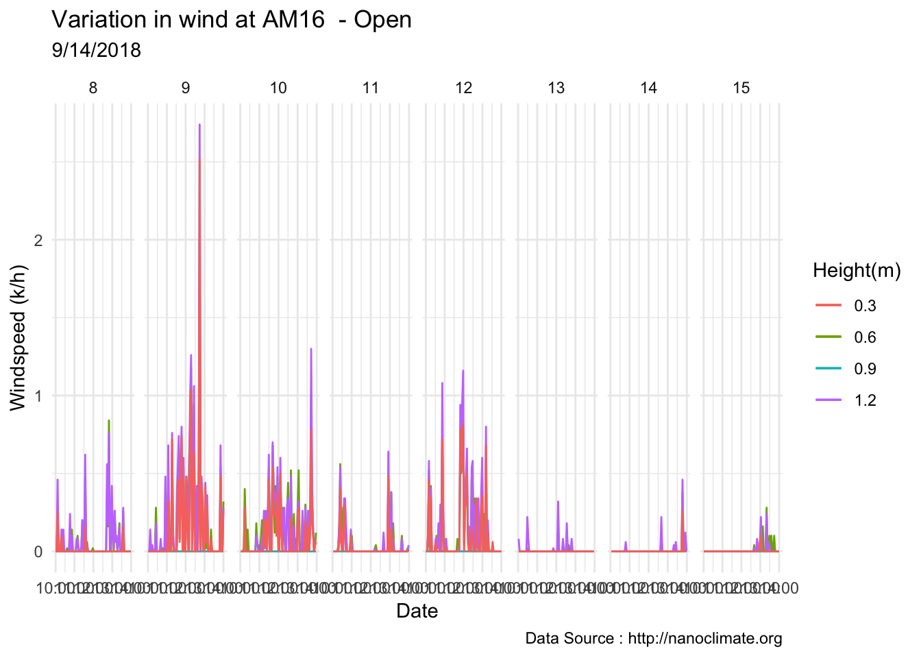
AG05
mclim_AG05_CN01_2018<-read_csv('./data/DATALOG-AG05-CN01.CSV')## Parsed with column specification:
## cols(
## date = col_character(),
## temp1 = col_double(),
## temp2 = col_double(),
## temp3 = col_double(),
## temp4 = col_double(),
## windspeed1 = col_double(),
## windspeed2 = col_double(),
## windspeed3 = col_double(),
## windspeed4 = col_double(),
## winddirection1 = col_double(),
## winddirection2 = col_double(),
## winddirection3 = col_double(),
## winddirection4 = col_double(),
## solar = col_double(),
## battery = col_double()
## )#mclim_AE10_CN01_2018<- read.csv('./data/DATALOG-AE10-CN01.CSV',stringsAsFactors = T)
names(mclim_AG05_CN01_2018)## [1] "date" "temp1" "temp2" "temp3"
## [5] "temp4" "windspeed1" "windspeed2" "windspeed3"
## [9] "windspeed4" "winddirection1" "winddirection2" "winddirection3"
## [13] "winddirection4" "solar" "battery"mclim_AG05_CN01_2018$time <- as_datetime(mclim_AG05_CN01_2018$date, format="%m/%d/%y %H:%M:%S",tz="America/Los_Angeles")
mclim_AG05_CN01_2018$time <-as.POSIXct(mclim_AG05_CN01_2018$time)
#Add hour month and day
## 11-05-2018
mclim_AG05_CN01_2018$hr <- hour(mclim_AG05_CN01_2018$time)
mclim_AG05_CN01_2018$minute <- minute(mclim_AG05_CN01_2018$time)
mclim_AG05_CN01_2018$day <- day(mclim_AG05_CN01_2018$time)
mclim_AG05_CN01_2018$month<- month(mclim_AG05_CN01_2018$time)
#Roughly one feet apart
mclim_AG05_CN01_2018$height <- 0
#therm1,28782877910A0217 - 0.6
#therm2,284CCE7791090235 - 1.2
#therm3,286C7A7791080217 - 0.9
#therm4,280A2577910A020D - 0.3
# mclim_AE10_CN01_2018[mclim_AE10_CN01_2018$nodeid=='2862367791040281' ,]$height <- 1.2
# mclim_AE10_CN01_2018[mclim_AE10_CN01_2018$nodeid=='286E9D77910802F2' ,]$height <- 0.6
# mclim_AE10_CN01_2018[mclim_AE10_CN01_2018$nodeid=='28A91B7791060263' ,]$height <- 0.3
# mclim_AE10_CN01_2018[mclim_AE10_CN01_2018$nodeid=='280704779106023F' ,]$height <- 0.9
## Day plot , Representive day
mclim_AG05_CN01_2018 %>% filter(month %in% c(9) & day(time) %in% c(10:20) & hr %in% c(10,11,12,13)) %>%
ggplot() + geom_line( aes(time,windspeed1,color = '0.6')) +
geom_line( aes(time,windspeed2,color = '1.2')) +
geom_line( aes(time,windspeed3,color = '0.9')) +
geom_line( aes(time,windspeed4,color = '0.3')) +
theme_minimal() +
facet_grid(. ~ day, scales = "free") +
ggtitle("Variation in wind at AG05 - Open") + xlab("Date") +
ylab("Windspeed (k/h)") + labs(colour = "Height(m)",
subtitle="9/14/2018",caption="Data Source : http://nanoclimate.org") 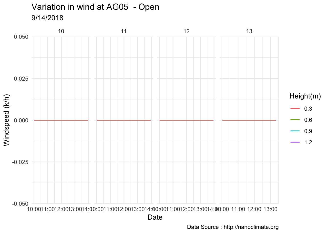
TO04
mclim_TO04_CN01_2018<-read_csv('./data/DATALOG-TO04-CN01.CSV')## Parsed with column specification:
## cols(
## date = col_character(),
## temp1 = col_double(),
## temp2 = col_double(),
## temp3 = col_double(),
## temp4 = col_double(),
## windspeed1 = col_double(),
## windspeed2 = col_double(),
## windspeed3 = col_double(),
## windspeed4 = col_double(),
## winddirection1 = col_double(),
## winddirection2 = col_double(),
## winddirection3 = col_double(),
## winddirection4 = col_double(),
## solar = col_double(),
## battery = col_double()
## )#mclim_AE10_CN01_2018<- read.csv('./data/DATALOG-AE10-CN01.CSV',stringsAsFactors = T)
names(mclim_TO04_CN01_2018)## [1] "date" "temp1" "temp2" "temp3"
## [5] "temp4" "windspeed1" "windspeed2" "windspeed3"
## [9] "windspeed4" "winddirection1" "winddirection2" "winddirection3"
## [13] "winddirection4" "solar" "battery"mclim_TO04_CN01_2018$time <- as_datetime(mclim_TO04_CN01_2018$date, format="%m/%d/%y %H:%M:%S",tz="America/Los_Angeles")
mclim_TO04_CN01_2018$time <-as.POSIXct(mclim_TO04_CN01_2018$time)
#Add hour month and day
## 11-05-2018
mclim_TO04_CN01_2018$hr <- hour(mclim_TO04_CN01_2018$time)
mclim_TO04_CN01_2018$minute <- minute(mclim_TO04_CN01_2018$time)
mclim_TO04_CN01_2018$day <- day(mclim_TO04_CN01_2018$time)
mclim_TO04_CN01_2018$month<- month(mclim_TO04_CN01_2018$time)
#Roughly one feet apart
mclim_TO04_CN01_2018$height <- 0
#therm1,28782877910A0217 - 0.6
#therm2,284CCE7791090235 - 1.2
#therm3,286C7A7791080217 - 0.9
#therm4,280A2577910A020D - 0.3
# mclim_AE10_CN01_2018[mclim_AE10_CN01_2018$nodeid=='2862367791040281' ,]$height <- 1.2
# mclim_AE10_CN01_2018[mclim_AE10_CN01_2018$nodeid=='286E9D77910802F2' ,]$height <- 0.6
# mclim_AE10_CN01_2018[mclim_AE10_CN01_2018$nodeid=='28A91B7791060263' ,]$height <- 0.3
# mclim_AE10_CN01_2018[mclim_AE10_CN01_2018$nodeid=='280704779106023F' ,]$height <- 0.9
## Day plot , Representive day
mclim_TO04_CN01_2018 %>% filter(month %in% c(9) & day(time) %in% c(5:10) & hr %in% c(10,11,12,13)) %>%
ggplot() + geom_line( aes(time,windspeed1,color = '0.6')) +
geom_line( aes(time,windspeed2,color = '1.2')) +
geom_line( aes(time,windspeed3,color = '0.9')) +
geom_line( aes(time,windspeed4,color = '0.3')) +
theme_minimal() +
facet_grid(. ~ day, scales = "free") +
ggtitle("Variation in wind at TO04 - Open") + xlab("Date") +
ylab("Windspeed (k/h)") + labs(colour = "Height(m)",
subtitle="9/14/2018",caption="Data Source : http://nanoclimate.org") 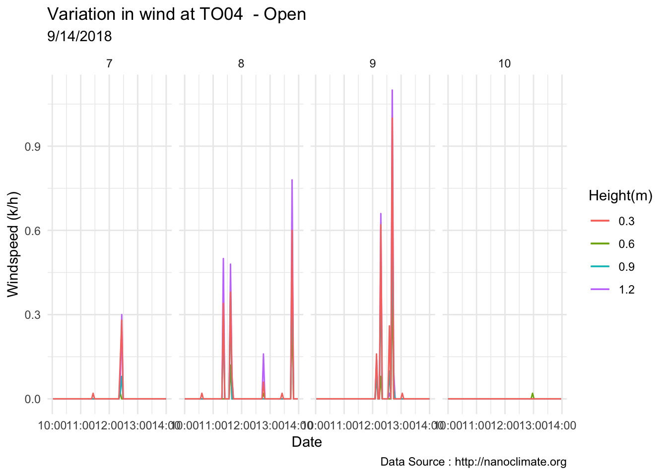
AM16
mclim_AM16_CN01_2018 %>% filter (!is.na(mclim_AM16_CN01_2018$minute) & month %in% c(9) ) %>%
filter( day %in% c(7:13)) %>%
mutate(solrf = ((solar-39) * 1.8) + ((25 -temp1) * .0012)) %>%
group_by(day,hr,minute) %>%
summarise(solmin = mean(solrf)) %>%
group_by(day,b = gl(ceiling(n()/4), 4, n())) %>%
group_by(day,hr,b) %>%
summarize(meansol = mean(solmin),
sd = sd(solmin)) %>%
mutate(height="1.2",newx= as.numeric(paste(hr,b,sep=""))) %>% #select(newx) %>% distinct(newx)
dplyr::group_by(day,height) %>%
mutate(index=1:n()) %>%
ggplot() +
geom_line(aes(index,meansol))+
theme_minimal() +
facet_grid(.~ day,scales = "free") +
scale_x_continuous(breaks = seq(0,119,by=1), limits = c(0,120),labels = labelfx) +
scale_colour_manual("Solar radiatiion on day", breaks = c("10","11", "12","13","14"), values = brewer.pal(5, "Set1")) +
scale_linetype_manual("Height(m)",values=c("1.2"=1)) +
theme_classic() + ggtitle("Diel Variation in radiation at 1.2m at site AM16") + xlab("Hour") +
ylab("Radiation (W/m^2)") + labs(colour = "Hour",
subtitle="9/9/18 - 9/12/19",caption="Data Source : http://www.nanoclimate.org") 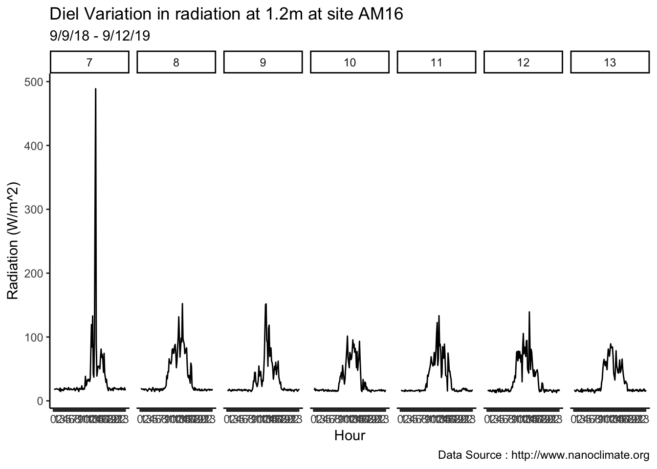
AG05
mclim_AG05_CN01_2018 %>% filter (!is.na(mclim_AG05_CN01_2018$minute) & month %in% c(9) ) %>%
filter( day %in% c(7:13)) %>%
mutate(solrf = ((solar-39) * 1.8) + ((25 -temp1) * .0012)) %>%
group_by(day,hr,minute) %>%
summarise(solmin = mean(solrf)) %>%
group_by(day,b = gl(ceiling(n()/4), 4, n())) %>%
group_by(day,hr,b) %>%
summarize(meansol = mean(solmin),
sd = sd(solmin)) %>%
mutate(height="1.2",newx= as.numeric(paste(hr,b,sep=""))) %>% #select(newx) %>% distinct(newx)
dplyr::group_by(day,height) %>%
mutate(index=1:n()) %>%
ggplot() +
geom_line(aes(index,meansol))+
theme_minimal() +
facet_grid(.~ day,scales = "free") +
scale_x_continuous(breaks = seq(0,119,by=1), limits = c(0,120),labels = labelfx) +
scale_colour_manual("Solar radiatiion on day", breaks = c("10","11", "12","13","14"), values = brewer.pal(5, "Set1")) +
scale_linetype_manual("Height(m)",values=c("1.2"=1)) +
theme_classic() + ggtitle("Diel Variation in radiation at 1.2m at site AG05") + xlab("Hour") +
ylab("Radiation (W/m^2)") + labs(colour = "Hour",
subtitle="9/9/18 - 9/12/19",caption="Data Source : http://www.nanoclimate.org") 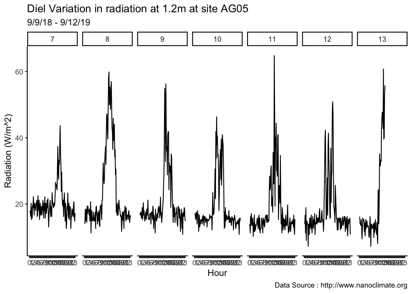
mclim_TO04_CN01_2018 %>% filter (!is.na(mclim_TO04_CN01_2018$minute) & month %in% c(9) ) %>%
filter( day %in% c(7:13)) %>%
mutate(solrf = ((solar-39) * 1.8) + ((25 -temp1) * .0012)) %>%
group_by(day,hr,minute) %>%
summarise(solmin = mean(solrf)) %>%
group_by(day,b = gl(ceiling(n()/4), 4, n())) %>%
group_by(day,hr,b) %>%
summarize(meansol = mean(solmin),
sd = sd(solmin)) %>%
mutate(height="1.2",newx= as.numeric(paste(hr,b,sep=""))) %>% #select(newx) %>% distinct(newx)
dplyr::group_by(day,height) %>%
mutate(index=1:n()) %>%
ggplot() +
geom_line(aes(index,meansol))+
theme_minimal() +
facet_grid(.~ day,scales = "free") +
scale_x_continuous(breaks = seq(0,119,by=1), limits = c(0,120),labels = labelfx) +
scale_colour_manual("Solar radiatiion on day", breaks = c("10","11", "12","13","14"), values = brewer.pal(5, "Set1")) +
scale_linetype_manual("Height(m)",values=c("1.2"=1)) +
theme_classic() + ggtitle("Diel Variation in radiation at 1.2m at site TO04") + xlab("Hour") +
ylab("Radiation (W/m^2)") + labs(colour = "Hour",
subtitle="9/9/18 - 9/12/19",caption="Data Source : http://www.nanoclimate.org") 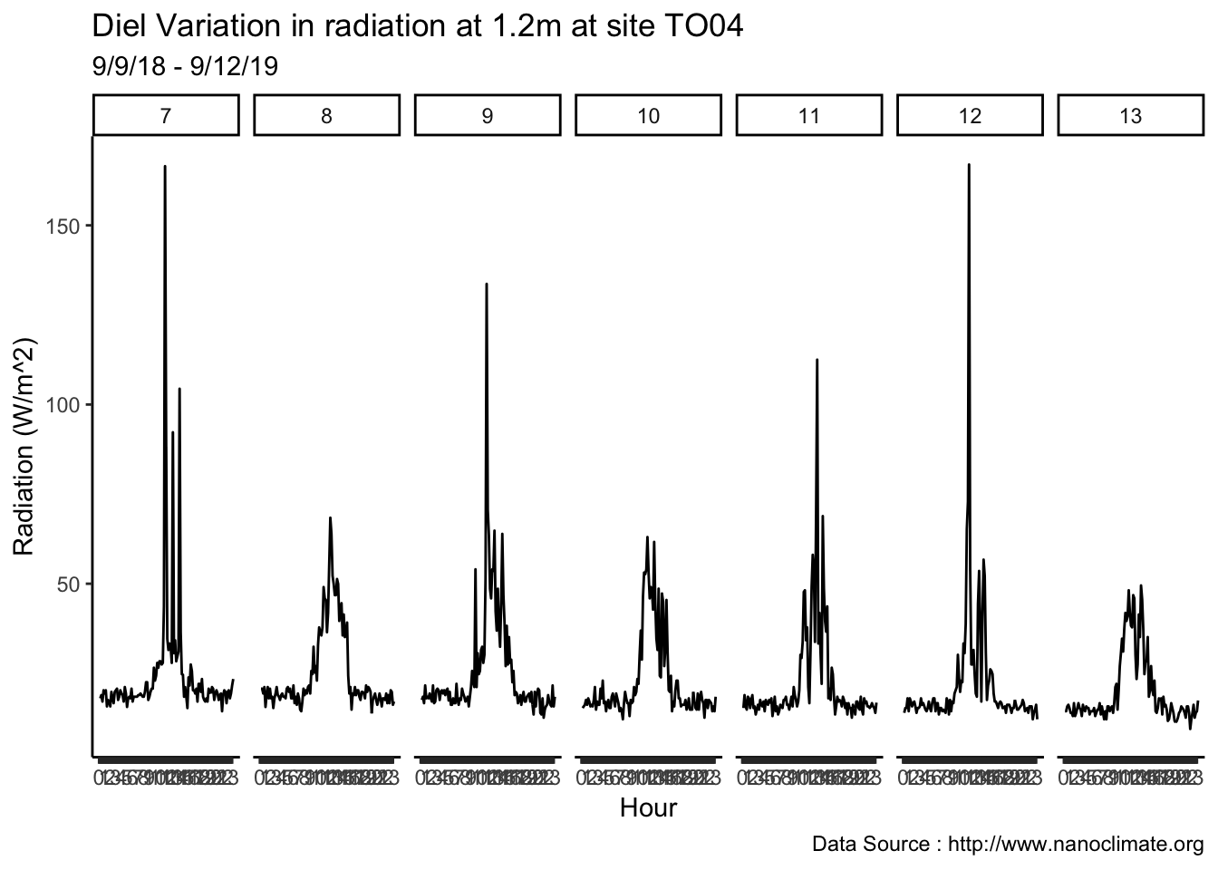
mclim_AE10_CN01_2018 %>% filter (!is.na(mclim_AE10_CN01_2018$minute) & month %in% c(9) ) %>%
filter( day %in% c(7:13)) %>%
mutate(solrf = ((solar-39) * 1.8) + ((25 -temp1) * .0012)) %>%
group_by(day,hr,minute) %>%
summarise(solmin = mean(solrf)) %>%
group_by(day,b = gl(ceiling(n()/4), 4, n())) %>%
group_by(day,hr,b) %>%
summarize(meansol = mean(solmin),
sd = sd(solmin)) %>%
mutate(height="1.2",newx= as.numeric(paste(hr,b,sep=""))) %>% #select(newx) %>% distinct(newx)
dplyr::group_by(day,height) %>%
mutate(index=1:n()) %>%
ggplot() +
geom_line(aes(index,meansol))+
theme_minimal() +
facet_grid(.~ day,scales = "free") +
scale_x_continuous(breaks = seq(0,119,by=1), limits = c(0,120),labels = labelfx) +
scale_colour_manual("Solar radiatiion on day", breaks = c("10","11", "12","13","14"), values = brewer.pal(5, "Set1")) +
scale_linetype_manual("Height(m)",values=c("1.2"=1)) +
theme_classic() + ggtitle("Diel Variation in radiation at 1.2m at site AE10") + xlab("Hour") +
ylab("Radiation (W/m^2)") + labs(colour = "Hour",
subtitle="9/9/18 - 9/12/19",caption="Data Source : http://www.nanoclimate.org") 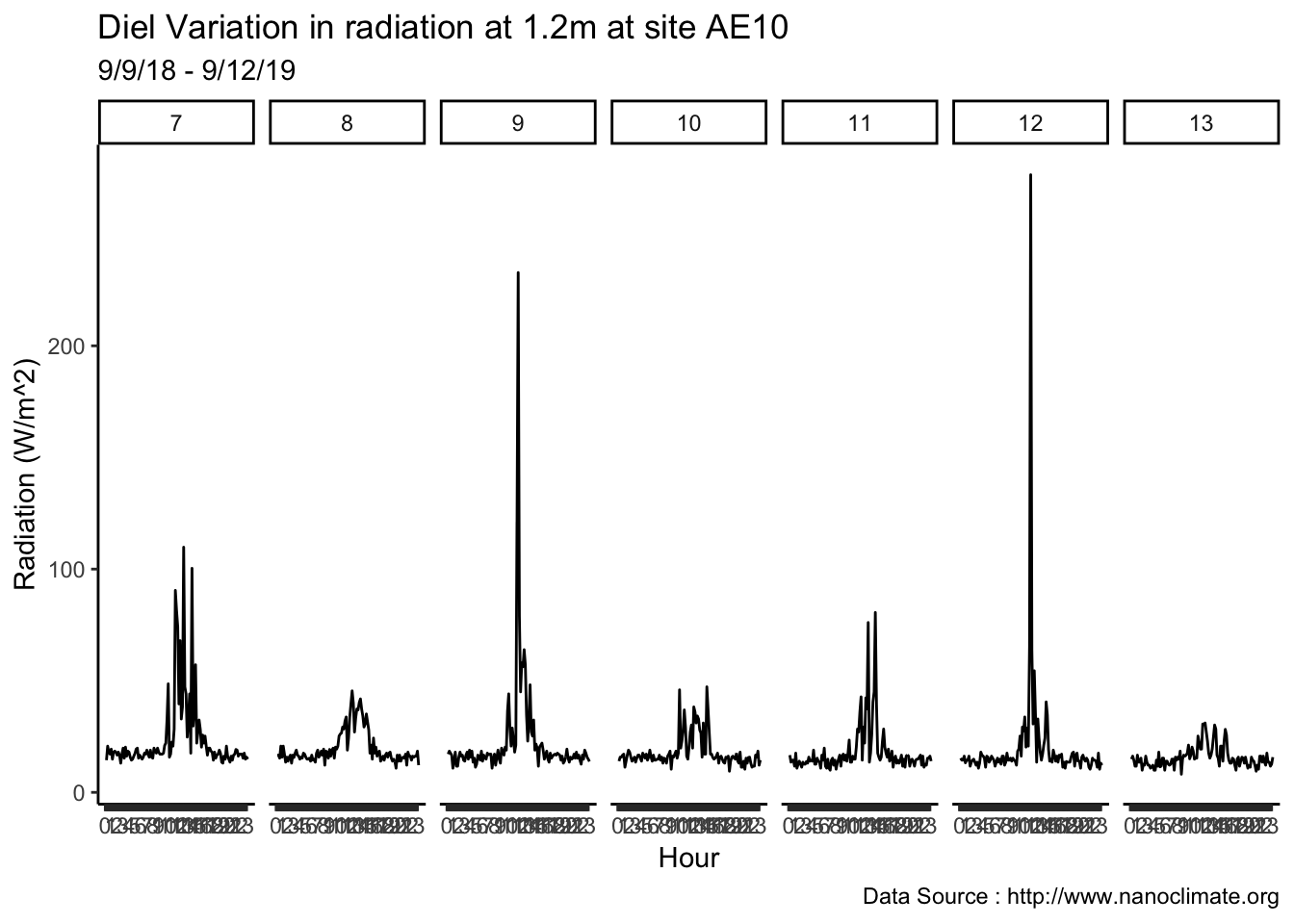
8.35 2-05-2019
Canopy reduces limits the amount of short-wave radiation ( Gay et al 1971, T R Oke BLC , P 125)
mclim_AE10_CN01_2018_solar <- mclim_AE10_CN01_2018 %>% filter (!is.na(mclim_AE10_CN01_2018$minute) & month %in% c(9) ) %>%
filter( day %in% c(7:13)) %>%
mutate(solrf = ((solar-39) * 1.8) + ((25 -temp1) * .0012)) %>%
group_by(day,hr,minute) %>%
summarise(solmin = mean(solrf)) %>%
group_by(day,b = gl(ceiling(n()/4), 4, n())) %>%
group_by(day,hr,b) %>%
summarize(meansol = mean(solmin),
sd = sd(solmin)) %>%
mutate(height="1.2",newx= as.numeric(paste(hr,b,sep=""))) %>% #select(newx) %>% distinct(newx)
dplyr::group_by(day,height) %>%
mutate(index=1:n()) %>% as.data.frame()
mclim_AE10_CN01_2018_solar$site <- 'AE10'
mclim_AM16_CN01_2018_solar <- mclim_AM16_CN01_2018 %>% filter (!is.na(mclim_AM16_CN01_2018$minute) & month %in% c(9) ) %>%
filter( day %in% c(7:13)) %>%
mutate(solrf = ((solar-39) * 1.8) + ((25 -temp1) * .0012)) %>%
group_by(day,hr,minute) %>%
summarise(solmin = mean(solrf)) %>%
group_by(day,b = gl(ceiling(n()/4), 4, n())) %>%
group_by(day,hr,b) %>%
summarize(meansol = mean(solmin),
sd = sd(solmin)) %>%
mutate(height="1.2",newx= as.numeric(paste(hr,b,sep=""))) %>% #select(newx) %>% distinct(newx)
dplyr::group_by(day,height) %>%
mutate(index=1:n()) %>% as.data.frame()
mclim_AM16_CN01_2018_solar$site <- 'AM16'
mclim_AG05_CN01_2018_solar <- mclim_AG05_CN01_2018 %>% filter (!is.na(mclim_AG05_CN01_2018$minute) & month %in% c(9) ) %>%
filter( day %in% c(7:13)) %>%
mutate(solrf = ((solar-39) * 1.8) + ((25 -temp1) * .0012)) %>%
group_by(day,hr,minute) %>%
summarise(solmin = mean(solrf)) %>%
group_by(day,b = gl(ceiling(n()/4), 4, n())) %>%
group_by(day,hr,b) %>%
summarize(meansol = mean(solmin),
sd = sd(solmin)) %>%
mutate(height="1.2",newx= as.numeric(paste(hr,b,sep=""))) %>% #select(newx) %>% distinct(newx)
dplyr::group_by(day,height) %>%
mutate(index=1:n()) %>% as.data.frame()
mclim_AG05_CN01_2018_solar$site <- 'AG05'
mclim_TO04_CN01_2018_solar <- mclim_TO04_CN01_2018 %>% filter (!is.na(mclim_TO04_CN01_2018$minute) & month %in% c(9) ) %>%
filter( day %in% c(7:13)) %>%
mutate(solrf = ((solar-39) * 1.8) + ((25 -temp1) * .0012)) %>%
group_by(day,hr,minute) %>%
summarise(solmin = mean(solrf)) %>%
group_by(day,b = gl(ceiling(n()/4), 4, n())) %>%
group_by(day,hr,b) %>%
summarize(meansol = mean(solmin),
sd = sd(solmin)) %>%
mutate(height="1.2",newx= as.numeric(paste(hr,b,sep=""))) %>% #select(newx) %>% distinct(newx)
dplyr::group_by(day,height) %>%
mutate(index=1:n()) %>% as.data.frame()
mclim_TO04_CN01_2018_solar$site <- 'TO04'
mclim_CN01_2018_solar_df <- rbind(mclim_AE10_CN01_2018_solar,
mclim_AM16_CN01_2018_solar,
mclim_AG05_CN01_2018_solar,
mclim_TO04_CN01_2018_solar)
mclim_CN01_2018_solar_df %>% filter(day %in% c(7:15)) %>%
ggplot() +
geom_line(aes(index,meansol,col=site))+
theme_minimal() +
facet_grid(.~ day,scales = "free") +
scale_x_continuous(breaks = seq(0,119,by=1), limits = c(0,120),labels = labelfx) +
scale_colour_manual("Solar radiatiion on day", values = brewer.pal(4, "Set1"),
labels=c('AE10 - 1450','AM16 - 1200','AG05 - 950','TO04 - 650')) +
scale_linetype_manual("Height(m)",values=c("1.2"=1)) +
theme_classic() + ggtitle("Diel Variation in radiation at 1.2m at 4 MM sites") + xlab("Hour") +
ylab("Radiation (W/m^2)") + labs(colour = "Hour",
subtitle="9/8/18 - 9/9/18",caption="Data Source : http://www.nanoclimate.org") 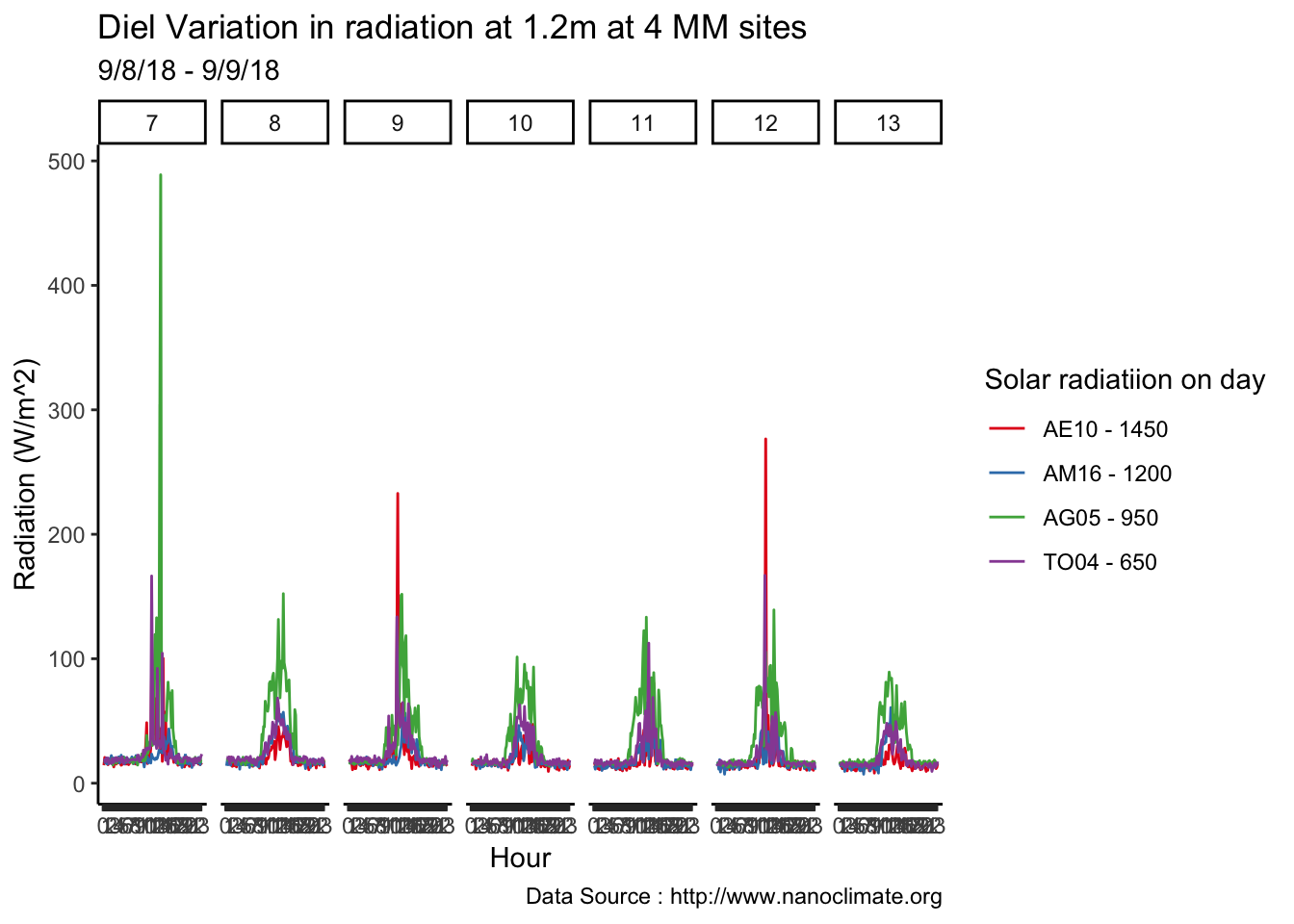
Plot wind for a day
mclim_CN01_2018_solar_df %>% filter(day %in% c(7:9)) %>%
ggplot() +
geom_line(aes(index,meansol,col=site))+
# theme_minimal() +
facet_grid(.~ day,scales = "free") +
scale_x_continuous(breaks = seq(0,119,by=1), limits = c(0,120),labels = labelfx) +
scale_colour_manual("Sites", values = brewer.pal(4, "Set1"),
labels=c('AE10 - 1450','AM16 - 1200','AG05 - 950','TO04 - 650')) +
scale_linetype_manual("Height(m)",values=c("1.2"=1)) +
theme_minimal(base_size=24) +
theme(legend.position = 'bottom',axis.text.x=element_text(angle=90)) +
ggtitle("Diel Variation in radiation at 1.2m at 4 MM sites") + xlab("Hour") +
ylab("Radiation (W/m^2)") + labs(colour = "Hour",
subtitle="",caption="Data Source : http://www.nanoclimate.org") 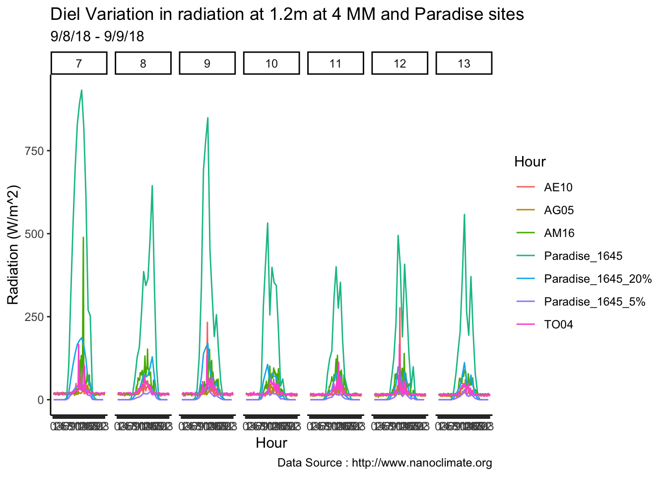
ggsave("mm_wind_evelation_1d.png",dpi=300, dev='png', height=8, width=16, units="in")Compare with Paradise
Try to plot with Paradise
Paradise_5to15_solar_df <- Paradise_5to15_solar %>%
filter (month %in% c(9) ) %>%
filter( day %in% c(7:13)) %>%
mutate(meansol=m1,b=0,sd=0,newx=0,height="1.2") %>%
dplyr::select(day,hr,sd,site,meansol,b,height,newx) %>%
dplyr::group_by(day) %>%
mutate(index= seq(1,120,by = 5)) %>%
dplyr::select(day,hr,b,meansol,sd,height,newx,index,site) %>% as.data.frame()
Paradise_5to15_solar_df_5pct <- Paradise_5to15_solar %>%
filter (month %in% c(9) ) %>%
filter( day %in% c(7:13)) %>%
mutate(meansol=m1*0.05,b=0,sd=0,newx=0,height="1.2") %>%
dplyr::select(day,hr,sd,site,meansol,b,height,newx) %>%
dplyr::group_by(day) %>%
mutate(index= seq(1,120,by = 5)) %>%
dplyr::select(day,hr,b,meansol,sd,height,newx,index,site) %>% as.data.frame()
Paradise_5to15_solar_df_5pct$site <- 'Paradise_1645_5%'
Paradise_5to15_solar_df_20pct <- Paradise_5to15_solar %>%
filter (month %in% c(9) ) %>%
filter( day %in% c(7:13)) %>%
mutate(meansol=m1*0.2,b=0,sd=0,newx=0,height="1.2") %>%
dplyr::select(day,hr,sd,site,meansol,b,height,newx) %>%
dplyr::group_by(day) %>%
mutate(index= seq(1,120,by = 5)) %>%
dplyr::select(day,hr,b,meansol,sd,height,newx,index,site) %>% as.data.frame()
Paradise_5to15_solar_df_20pct$site <- 'Paradise_1645_20%'
mclim_CN01_2018_solar_df_compare <- rbind(mclim_AE10_CN01_2018_solar,
mclim_AM16_CN01_2018_solar,
mclim_AG05_CN01_2018_solar,
mclim_TO04_CN01_2018_solar,
Paradise_5to15_solar_df,
Paradise_5to15_solar_df_5pct,
Paradise_5to15_solar_df_20pct)
mclim_CN01_2018_solar_df_compare %>% filter(day %in% c(5:15)) %>%
ggplot() +
geom_line(aes(index,meansol,col=site))+
theme_minimal() +
facet_grid(.~ day,scales = "free") +
scale_x_continuous(breaks = seq(0,119,by=1), limits = c(0,120),labels = labelfx) +
# scale_colour_manual("Solar radiatiion on day", values = brewer.pal(7, "Set1"),
# labels=c('AE10 - 1450','AM16 - 1200','AG05 - 950','TO04 - 650','Paradise - 1645','Paradise - 1645_5%','Paradise - 1645_20%')) +
scale_linetype_manual("Height(m)",values=c("1.2"=1)) +
theme_classic() + ggtitle("Diel Variation in radiation at 1.2m at 4 MM and Paradise sites") + xlab("Hour") +
ylab("Radiation (W/m^2)") + labs(colour = "Hour",
subtitle="9/8/18 - 9/9/18",caption="Data Source : http://www.nanoclimate.org") 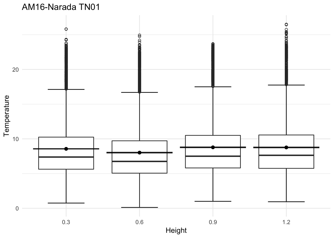
8.36 2-23-2019
Looking at the variation by height at each individual heights, expect it to be variable closer to ground. More turbulent
AM16 - TN01
ggplot(mclim_AM16_TN01_2018, aes(as.factor(height), temp))+
stat_boxplot( aes(as.factor(height), temp),
geom='errorbar', linetype=1, width=0.5)+ #whiskers
geom_boxplot( aes(as.factor(height), temp),outlier.shape=1) +
stat_summary(fun.y=mean, geom="point", size=2) +
stat_summary(fun.data = mean_se, geom = "errorbar") +
theme_minimal() +
ylab("Temperature") + xlab("Height") +ggtitle("AM16-Narada TN01") 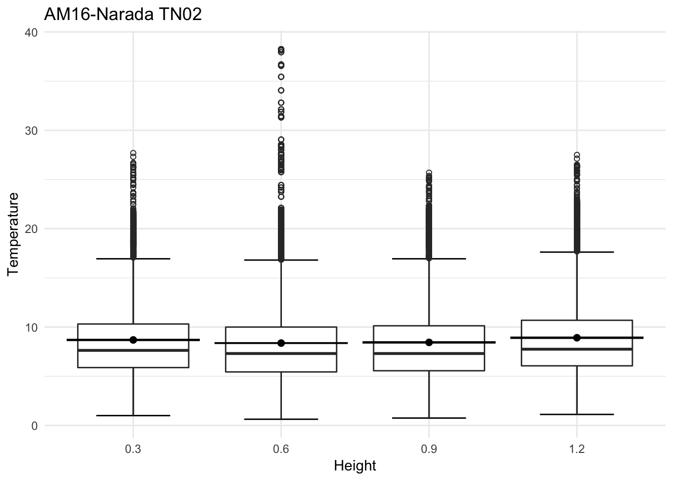 TN02
TN02
ggplot(mclim_AM16_TN02_2018, aes(as.factor(height), temp))+
stat_boxplot( aes(as.factor(height), temp),
geom='errorbar', linetype=1, width=0.5)+ #whiskers
geom_boxplot( aes(as.factor(height), temp),outlier.shape=1) +
stat_summary(fun.y=mean, geom="point", size=2) +
stat_summary(fun.data = mean_se, geom = "errorbar") +
theme_minimal() +
ylab("Temperature") + xlab("Height") +ggtitle("AM16-Narada TN02") 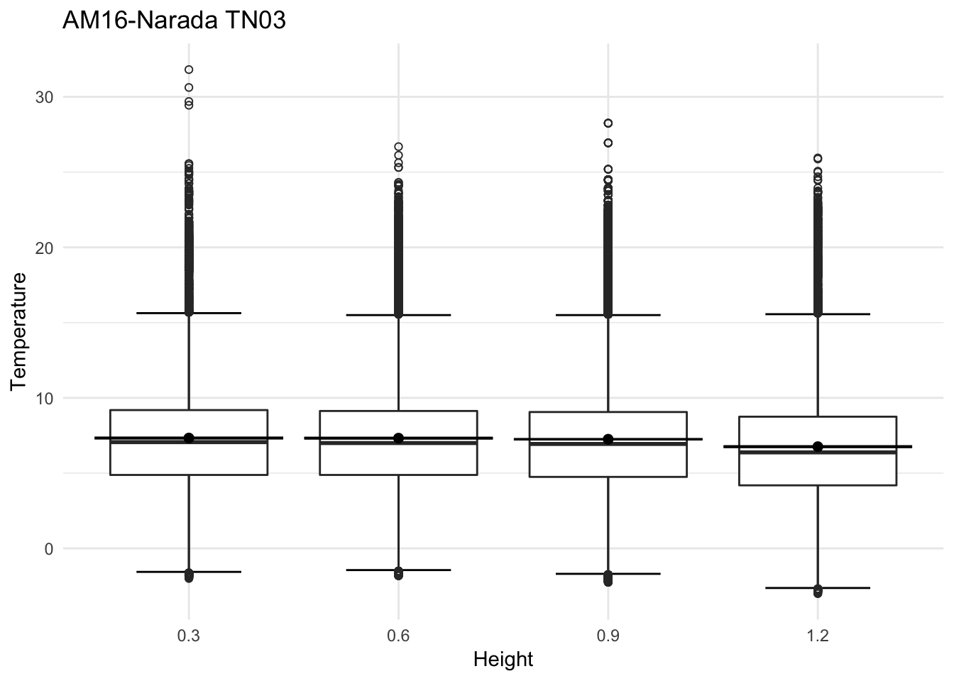 TN03
TN03
mclim_AM16_TN03_2018 %>%
filter(height > 0) %>%
ggplot( aes(as.factor(height), temp))+
stat_boxplot( aes(as.factor(height), temp),
geom='errorbar', linetype=1, width=0.5)+ #whiskers
geom_boxplot( aes(as.factor(height), temp),outlier.shape=1) +
stat_summary(fun.y=mean, geom="point", size=2) +
stat_summary(fun.data = mean_se, geom = "errorbar") +
theme_minimal() +
ylab("Temperature") + xlab("Height") +ggtitle("AM16-Narada TN03") 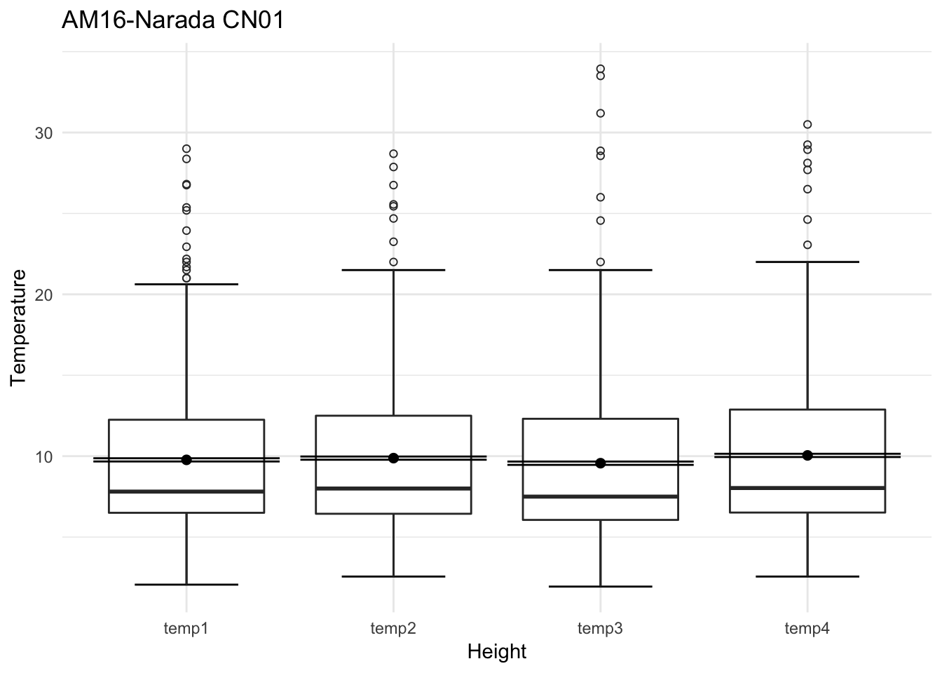
AM16 CN01
mclim_AM16_CN01_2018 %>% dplyr::select(time, temp1,temp2,temp3,temp4) %>%
dplyr::filter(temp1 >0 & temp2 >0 & temp3 >0 & temp4 > 0 ) %>%
dplyr::filter(temp1 <50 & temp2 <50 & temp3 <50 & temp4 < 50 ) %>%
gather(variable, value,-time) %>%
ggplot( aes(as.factor(variable), value))+
stat_boxplot( aes(as.factor(variable), value),
geom='errorbar', linetype=1, width=0.5)+ #whiskers
geom_boxplot( aes(as.factor(variable), value),outlier.shape=1) +
stat_summary(fun.y=mean, geom="point", size=2) +
stat_summary(fun.data = mean_se, geom = "errorbar") +
theme_minimal() +
ylab("Temperature") + xlab("Height") +ggtitle("AM16-Narada CN01") 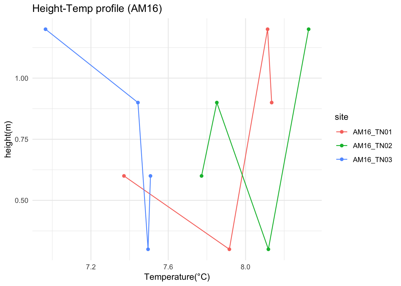
Do Z-Temp profile for AM16
mclim_AM16_TN01_2018_ZT <- mclim_AM16_TN01_2018
mclim_AM16_TN01_2018_ZT$site <- 'AM16_TN01'
mclim_AM16_TN01_2018_ZT$canopy <- 'Closed'
mclim_AM16_TN02_2018_ZT <- mclim_AM16_TN02_2018
mclim_AM16_TN02_2018_ZT$site <- 'AM16_TN02'
mclim_AM16_TN02_2018_ZT$canopy <- 'Closed'
mclim_AM16_TN03_2018_ZT <- mclim_AM16_TN03_2018
mclim_AM16_TN03_2018_ZT$site <- 'AM16_TN03'
mclim_AM16_TN03_2018_ZT$canopy <- 'Open'
mclim_AM16_2018_ZTemp<- rbind(mclim_AM16_TN01_2018_ZT,
mclim_AM16_TN02_2018_ZT,
mclim_AM16_TN03_2018_ZT
)
mclim_AM16_2018_ZTemp %>% dplyr::filter(height > 0 & day >5) %>%
dplyr::group_by (site,height ) %>%
dplyr::summarise(meant=mean(temp))%>%
ggplot( )+
geom_point(aes(meant,height,color=site)) +
geom_line(aes(meant,height,color=site)) +
#geom_smooth(span = .4,aes(meant,height,color=site)) +
theme_minimal() +
ylab("height(m)") + xlab("Temperature(°C)") +ggtitle("Height-Temp profile (AM16)") 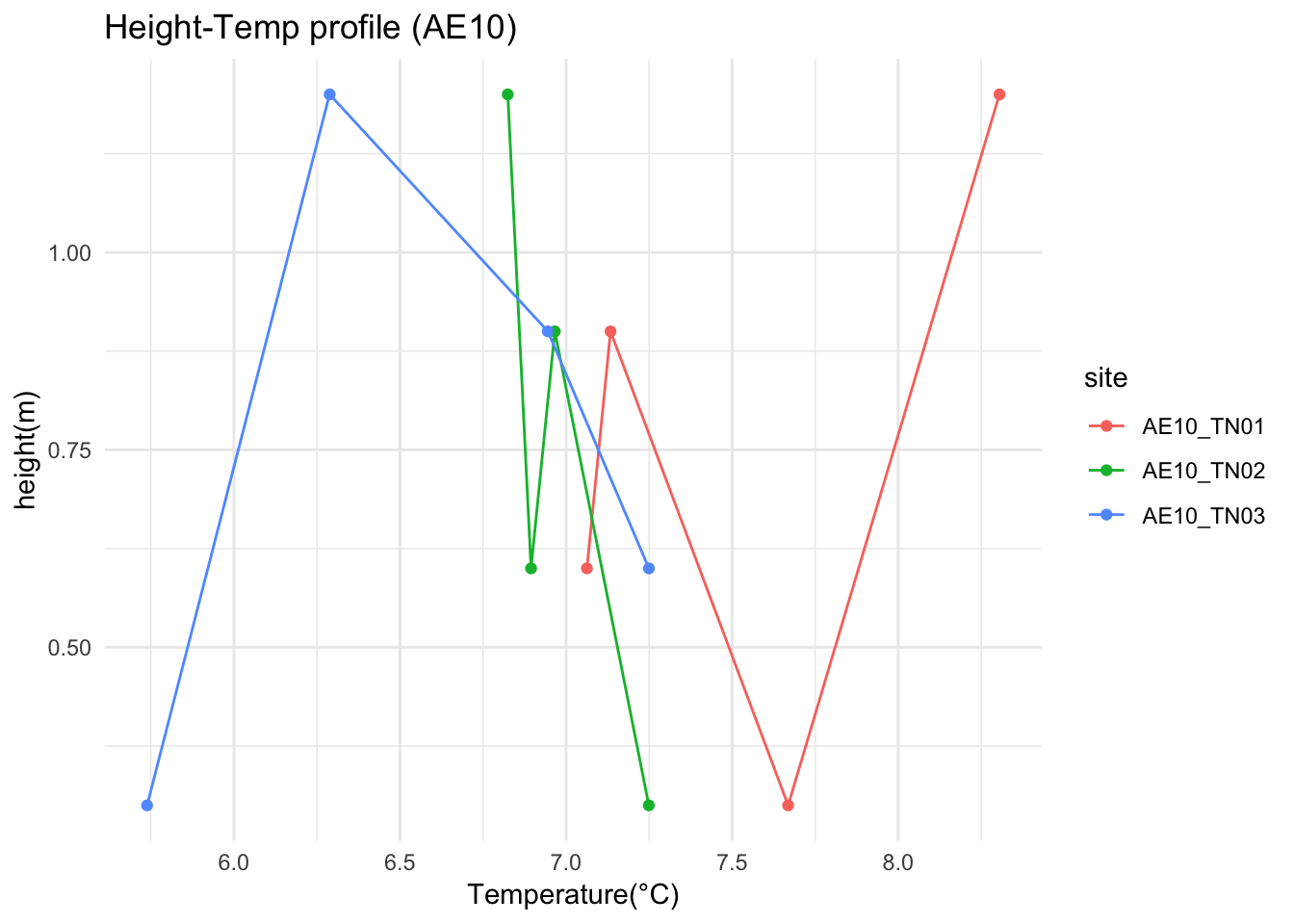
Do Z-Temp profile for AE10
mclim_AE10_TN01_2018_ZT <- mclim_AE10_TN01_2018
mclim_AE10_TN01_2018_ZT$site <- 'AE10_TN01'
mclim_AE10_TN01_2018_ZT$canopy <- 'Open'
mclim_AE10_TN02_2018_ZT <- mclim_AE10_TN02_2018
mclim_AE10_TN02_2018_ZT$site <- 'AE10_TN02'
mclim_AE10_TN02_2018_ZT$canopy <- 'Closed'
mclim_AE10_TN03_2018_ZT <- mclim_AE10_TN03_2018
mclim_AE10_TN03_2018_ZT$site <- 'AE10_TN03'
mclim_AE10_TN03_2018_ZT$canopy <- 'Closed'
mclim_AE10_2018_ZTemp<- rbind(mclim_AE10_TN01_2018_ZT,
mclim_AE10_TN02_2018_ZT,
mclim_AE10_TN03_2018_ZT
)
mclim_AE10_2018_ZTemp %>% dplyr::filter(height > 0 & temp >0 & day >5) %>%
dplyr::group_by (site,height ) %>%
dplyr::summarise(meant=mean(temp))%>%
ggplot( )+
geom_point(aes(meant,height,color=site)) +
geom_line(aes(meant,height,color=site)) +
theme_minimal() +
ylab("height(m)") + xlab("Temperature(°C)") +ggtitle("Height-Temp profile (AE10)") 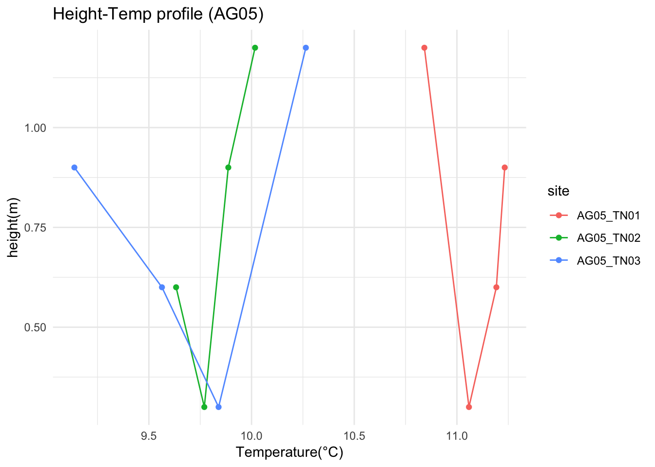 AG05
AG05
mclim_AG05_TN01_2018_ZT <- mclim_AG05_TN01_2018
mclim_AG05_TN01_2018_ZT$site <- 'AG05_TN01'
mclim_AG05_TN01_2018_ZT$canopy <- 'Closed'
mclim_AG05_TN02_2018_ZT <- mclim_AG05_TN02_2018
mclim_AG05_TN02_2018_ZT$site <- 'AG05_TN02'
mclim_AG05_TN02_2018_ZT$canopy <- 'Closed'
mclim_AG05_TN03_2018_ZT <- mclim_AG05_TN03_2018
mclim_AG05_TN03_2018_ZT$site <- 'AG05_TN03'
mclim_AG05_TN03_2018_ZT$canopy <- 'Open'
mclim_AG05_2018_ZTemp<- rbind(mclim_AG05_TN01_2018_ZT,
mclim_AG05_TN02_2018_ZT,
mclim_AG05_TN03_2018_ZT
)
mclim_AG05_2018_ZTemp %>% dplyr::filter(height > 0 & temp >0 & day >5) %>%
dplyr::group_by (site,height ) %>%
dplyr::summarise(meant=mean(temp))%>%
ggplot( )+
geom_point(aes(meant,height,color=site)) +
geom_line(aes(meant,height,color=site)) +
theme_minimal() +
ylab("height(m)") + xlab("Temperature(°C)") +ggtitle("Height-Temp profile (AG05)") 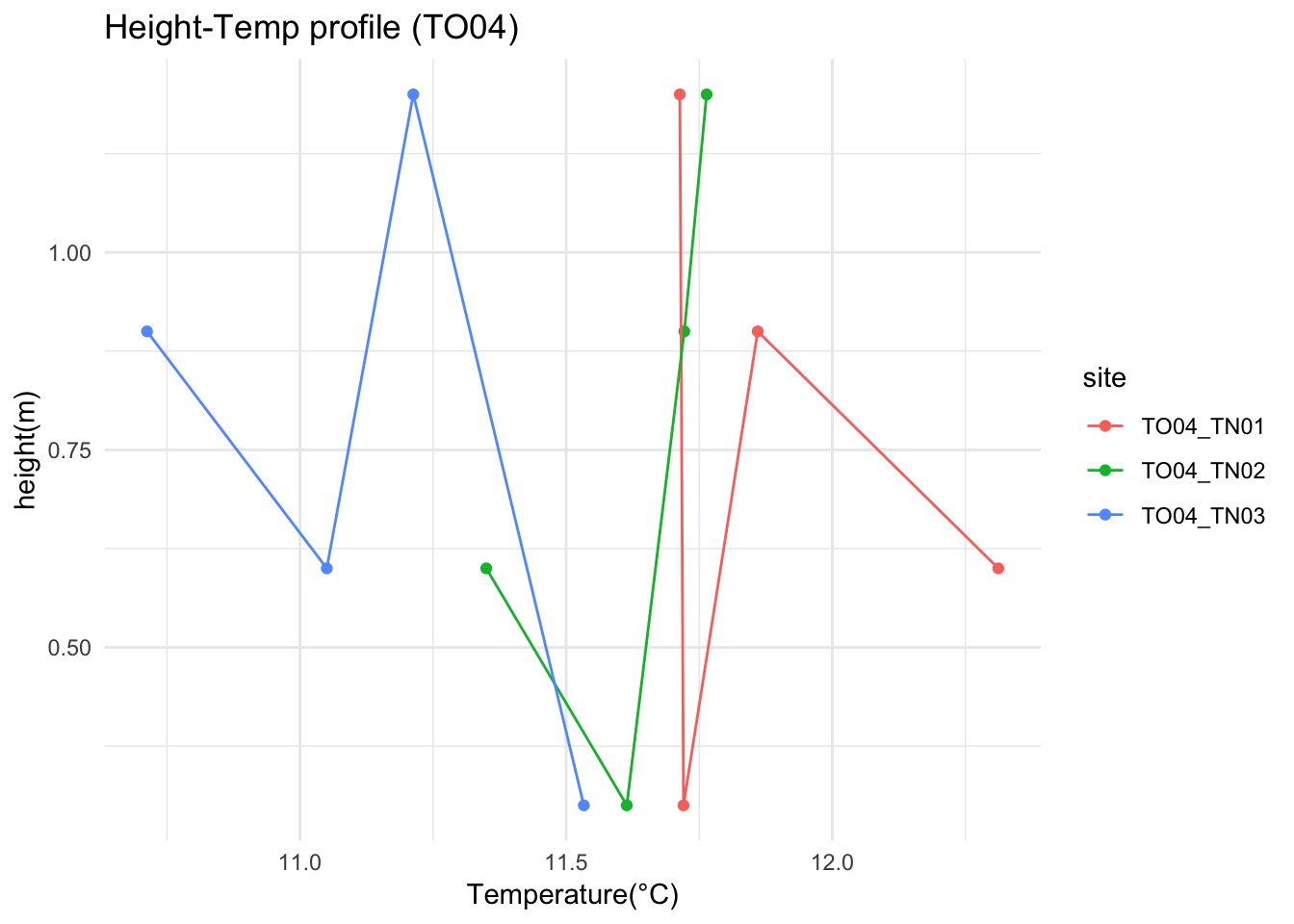 TO04
TO04
mclim_TO04_TN01_2018_ZT <- mclim_TO04_TN01_2018
mclim_TO04_TN01_2018_ZT$site <- 'TO04_TN01'
mclim_TO04_TN01_2018_ZT$canopy <- 'Closed'
mclim_TO04_TN02_2018_ZT <- mclim_TO04_TN02_2018
mclim_TO04_TN02_2018_ZT$site <- 'TO04_TN02'
mclim_TO04_TN02_2018_ZT$canopy <- 'Open'
mclim_TO04_TN03_2018_ZT <- mclim_TO04_TN03_2018
mclim_TO04_TN03_2018_ZT$site <- 'TO04_TN03'
mclim_TO04_TN03_2018_ZT$canopy <- 'Closed'
mclim_TO04_2018_ZTemp<- rbind(mclim_TO04_TN01_2018_ZT,
mclim_TO04_TN02_2018_ZT,
mclim_TO04_TN03_2018_ZT
)
mclim_TO04_2018_ZTemp %>% dplyr::filter(height > 0 & temp >0 & day >5) %>%
dplyr::group_by (site,height ) %>%
dplyr::summarise(meant=mean(temp))%>%
ggplot( )+
geom_point(aes(meant,height,color=site)) +
geom_line(aes(meant,height,color=site)) +
theme_minimal() +
ylab("height(m)") + xlab("Temperature(°C)") +ggtitle("Height-Temp profile (TO04)") 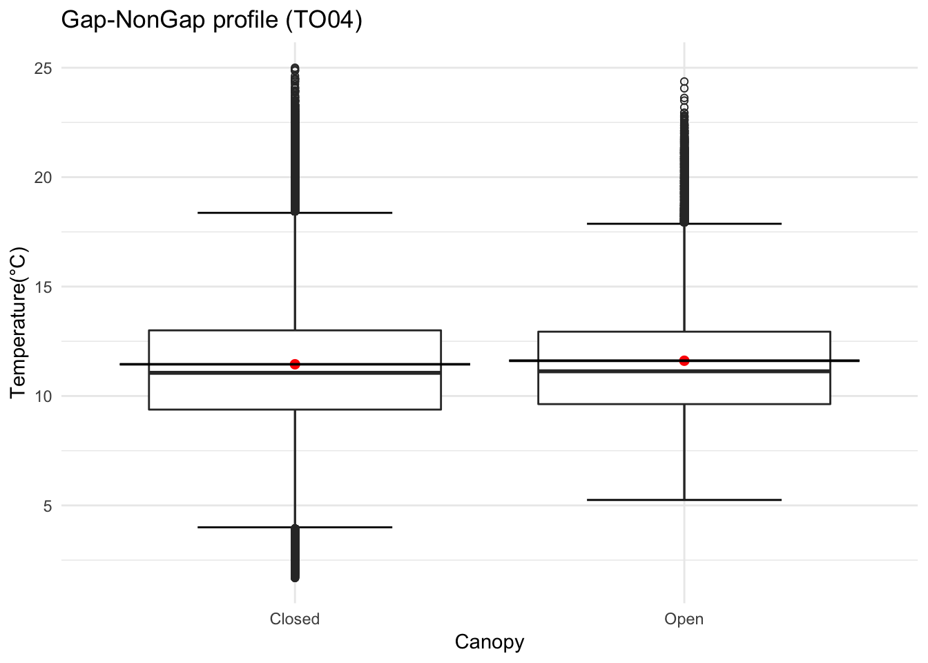 Gap and non gap
` TO04
mclim_TO04_2018_ZTemp %>% dplyr::filter(height > 0 & temp >0 & day >5) %>%
ggplot( aes(as.factor(canopy), temp))+
stat_boxplot( aes(as.factor(canopy), temp),
geom='errorbar', linetype=1, width=0.5)+ #whiskers
geom_boxplot( aes(as.factor(canopy), temp),outlier.shape=1) +
stat_summary(fun.y=mean, geom="point", size=2,color="red") +
stat_summary(fun.data = mean_se, geom = "errorbar") +
theme_minimal() +
ylab("Temperature(°C)") + xlab("Canopy") +ggtitle("Gap-NonGap profile (TO04)") 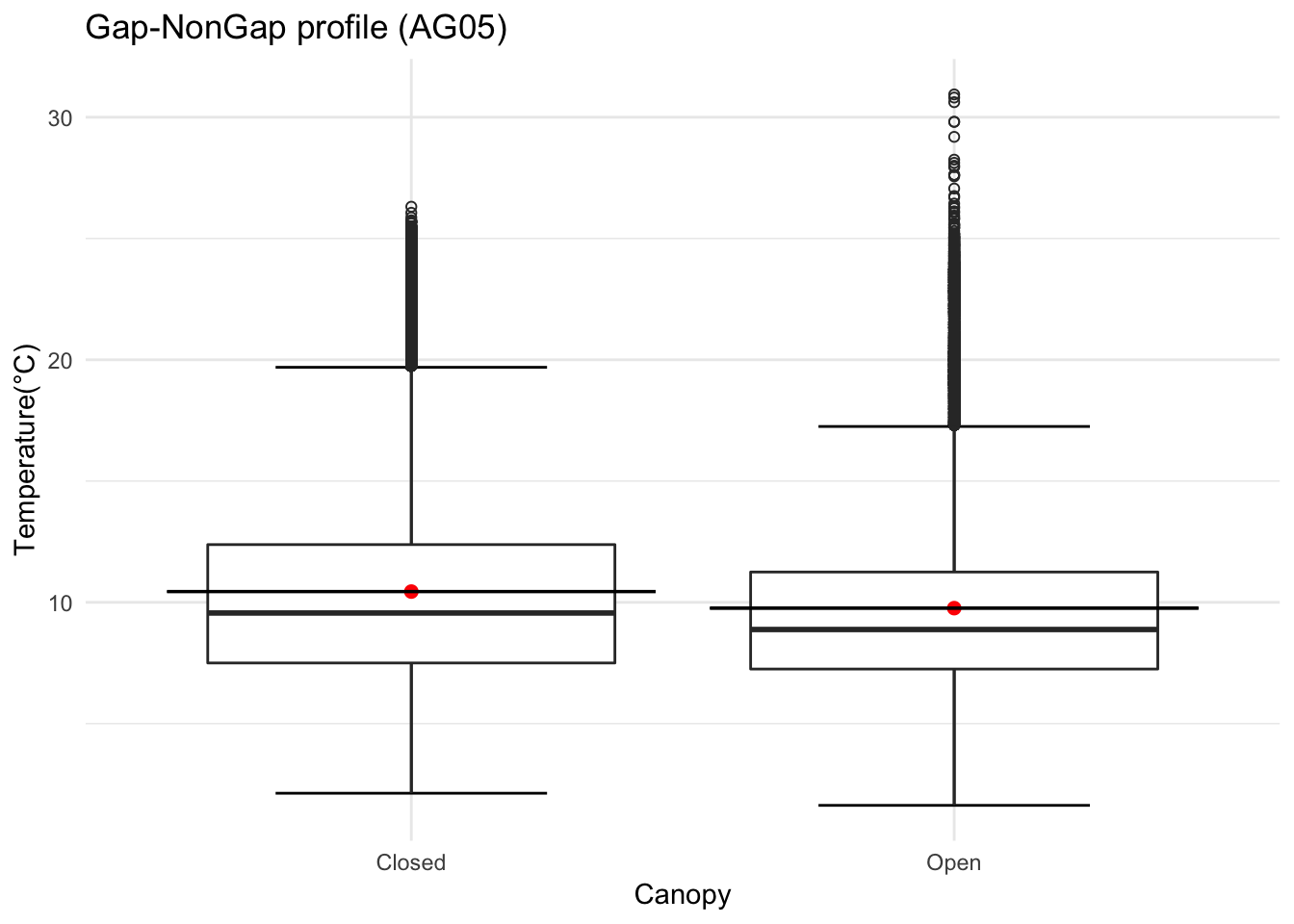
AG05
mclim_AG05_2018_ZTemp %>% dplyr::filter(height > 0 & temp >0 & day >5) %>%
ggplot( aes(as.factor(canopy), temp))+
stat_boxplot( aes(as.factor(canopy), temp),
geom='errorbar', linetype=1, width=0.5)+ #whiskers
geom_boxplot( aes(as.factor(canopy), temp),outlier.shape=1) +
stat_summary(fun.y=mean, geom="point", size=2,color="red") +
stat_summary(fun.data = mean_se, geom = "errorbar") +
theme_minimal() +
ylab("Temperature(°C)") + xlab("Canopy") +ggtitle("Gap-NonGap profile (AG05)") 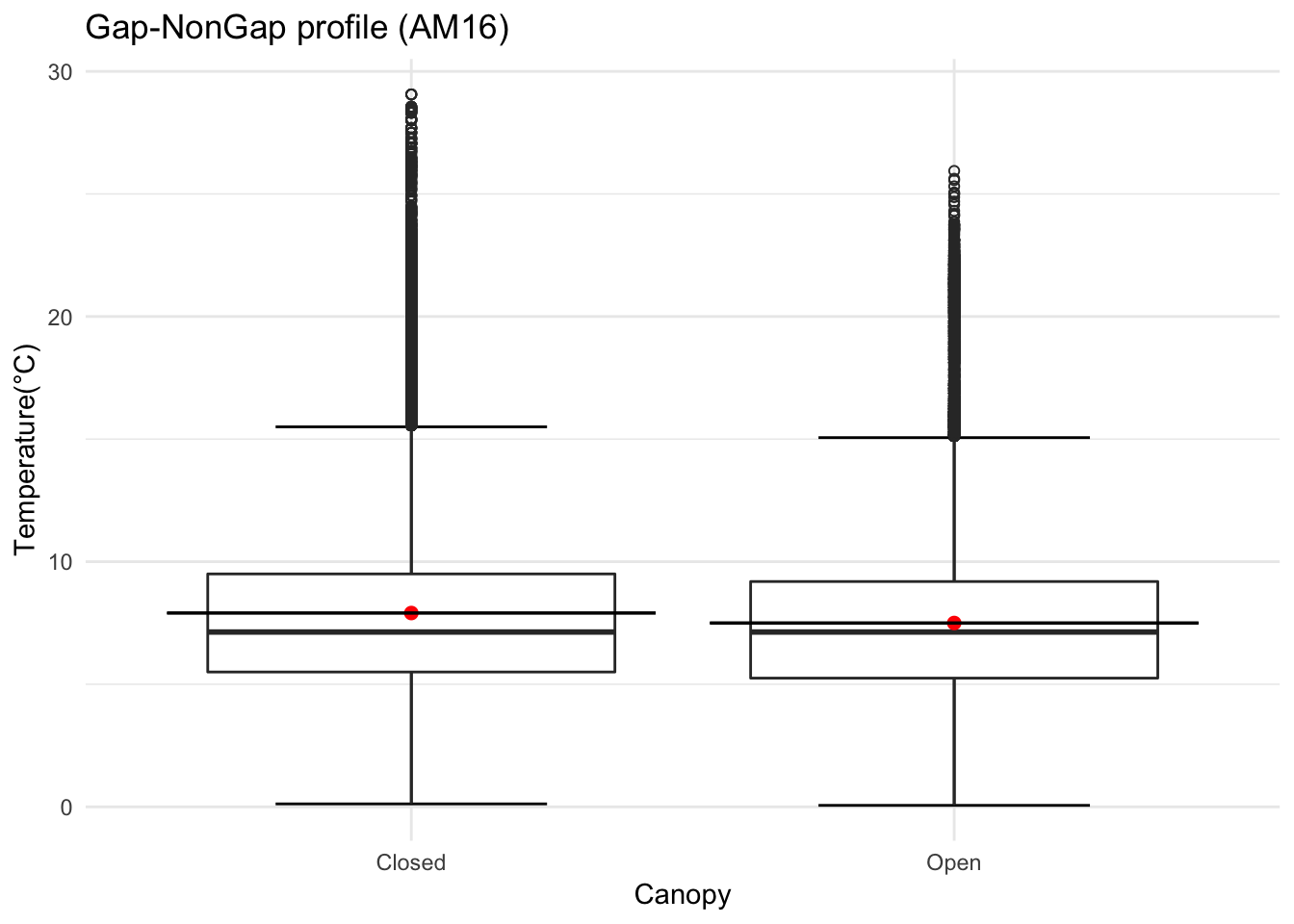 AM16
AM16
mclim_AM16_2018_ZTemp %>% dplyr::filter(height > 0 & temp >0 & day >5) %>%
ggplot( aes(as.factor(canopy), temp))+
stat_boxplot( aes(as.factor(canopy), temp),
geom='errorbar', linetype=1, width=0.5)+ #whiskers
geom_boxplot( aes(as.factor(canopy), temp),outlier.shape=1) +
stat_summary(fun.y=mean, geom="point", size=2,color="red") +
stat_summary(fun.data = mean_se, geom = "errorbar") +
theme_minimal() +
ylab("Temperature(°C)") + xlab("Canopy") +ggtitle("Gap-NonGap profile (AM16)") 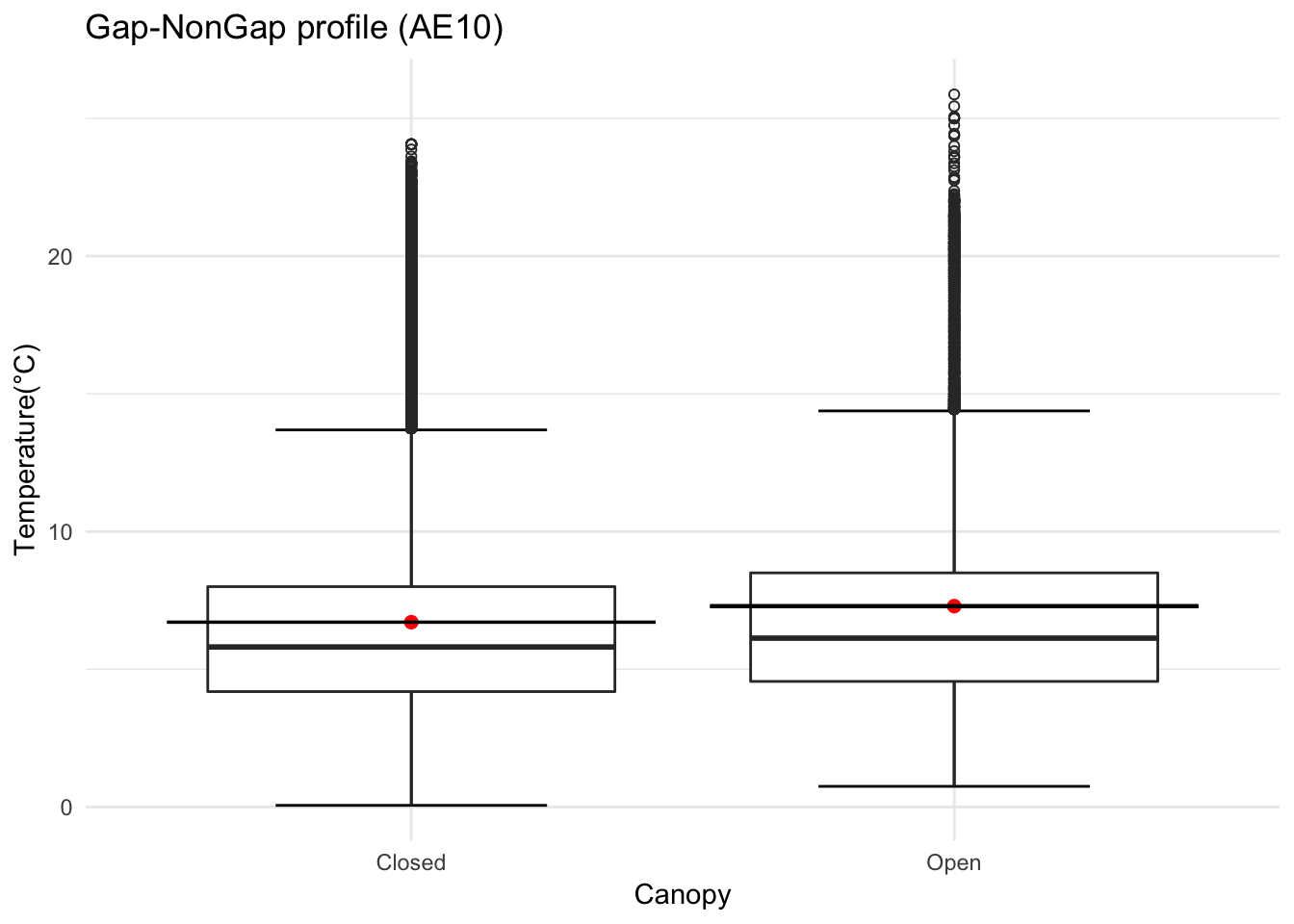
AE10
mclim_AE10_2018_ZTemp %>% dplyr::filter(height > 0 & temp >0 & day >5) %>%
ggplot( aes(as.factor(canopy), temp))+
stat_boxplot( aes(as.factor(canopy), temp),
geom='errorbar', linetype=1, width=0.5)+ #whiskers
geom_boxplot( aes(as.factor(canopy), temp),outlier.shape=1) +
stat_summary(fun.y=mean, geom="point", size=2,color="red") +
stat_summary(fun.data = mean_se, geom = "errorbar") +
theme_minimal() +
ylab("Temperature(°C)") + xlab("Canopy") +ggtitle("Gap-NonGap profile (AE10)") 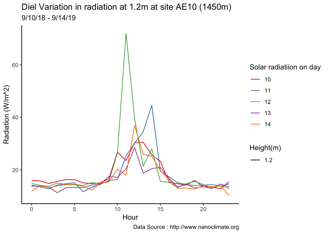
Onto Radiation (redo), use AE10-CN01
mclim_AE10_CN01_2018 %>% filter (!is.na(mclim_AE10_CN01_2018$minute) & month %in% c(9) ) %>%
filter( day > 9 & day < 15) %>%
mutate(solrf = ((solar-39) * 1.8) + ((25 -temp1) * .0012)) %>%
group_by(month,day,hr) %>%
add_count(wt=3) %>%
summarise(m1= mean(solrf)) %>%
group_by(day,hr) %>%
ggplot() +
geom_line(aes(hr,m1,group=day ,color=as.factor(day),linetype = '1.2'),se=F)+
scale_colour_manual("Solar radiatiion on day", breaks = c("10","11", "12","13","14"), values = brewer.pal(5, "Set1")) +
scale_linetype_manual("Height(m)",values=c("1.2"=1)) +
theme_classic() + ggtitle("Diel Variation in radiation at 1.2m at site AE10 (1450m)") + xlab("Hour") +
ylab("Radiation (W/m^2)") + labs(colour = "Hour",
subtitle="9/10/18 - 9/14/19",caption="Data Source : http://www.nanoclimate.org") 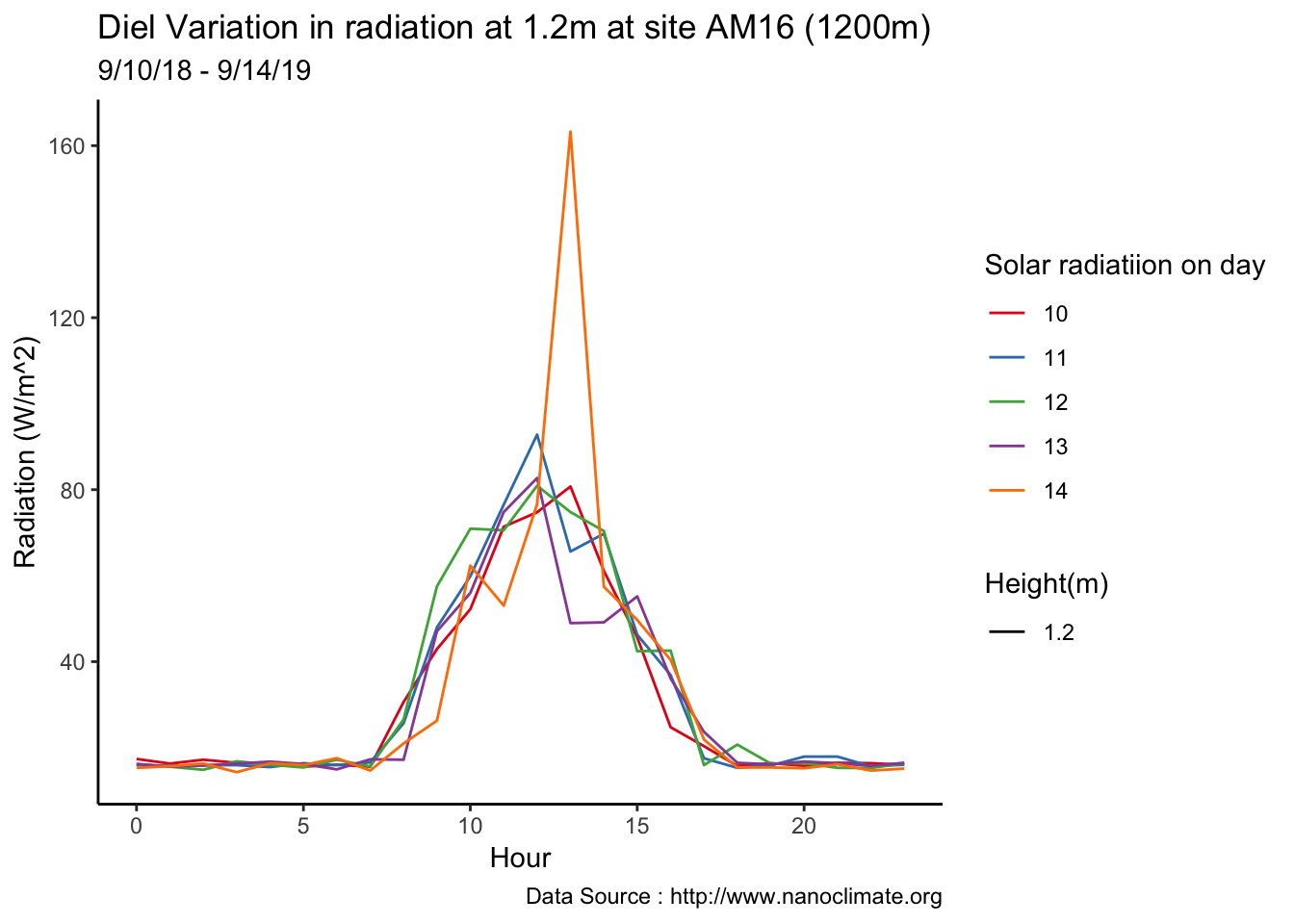
AM16
mclim_AM16_CN01_2018 %>% filter (!is.na(mclim_AM16_CN01_2018$minute) & month %in% c(9) ) %>%
filter( day > 9 & day < 15) %>%
mutate(solrf = ((solar-39) * 1.8) + ((25 -temp1) * .0012)) %>%
group_by(month,day,hr) %>%
add_count(wt=3) %>%
summarise(m1= mean(solrf)) %>%
group_by(day,hr) %>%
ggplot() +
geom_line(aes(hr,m1,group=day ,color=as.factor(day),linetype = '1.2'),se=F)+
scale_colour_manual("Solar radiatiion on day", breaks = c("10","11", "12","13","14"), values = brewer.pal(5, "Set1")) +
scale_linetype_manual("Height(m)",values=c("1.2"=1)) +
theme_classic() + ggtitle("Diel Variation in radiation at 1.2m at site AM16 (1200m)") + xlab("Hour") +
ylab("Radiation (W/m^2)") + labs(colour = "Hour",
subtitle="9/10/18 - 9/14/19",caption="Data Source : http://www.nanoclimate.org") 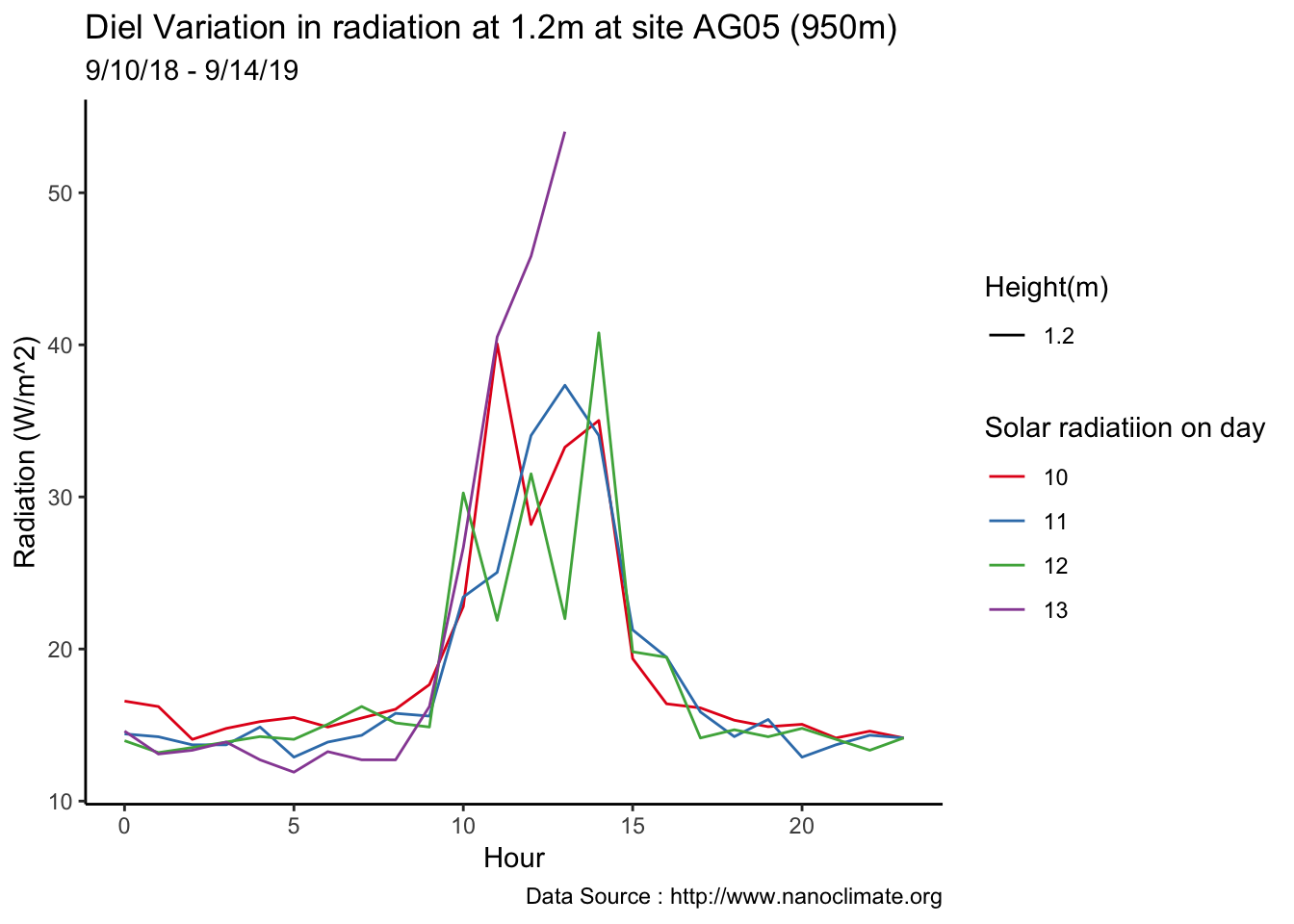 AG05 - Missed data
mclim_AG05_CN01_2018 %>% filter (!is.na(mclim_AG05_CN01_2018$minute) & month %in% c(9) ) %>%
filter( day > 9 & day < 15) %>%
mutate(solrf = ((solar-39) * 1.8) + ((25 -temp1) * .0012)) %>%
group_by(month,day,hr) %>%
add_count(wt=3) %>%
summarise(m1= mean(solrf)) %>%
group_by(day,hr) %>%
ggplot() +
geom_line(aes(hr,m1,group=day ,color=as.factor(day),linetype = '1.2'),se=F)+
scale_colour_manual("Solar radiatiion on day", breaks = c("10","11", "12","13","14"), values = brewer.pal(5, "Set1")) +
scale_linetype_manual("Height(m)",values=c("1.2"=1)) +
theme_classic() + ggtitle("Diel Variation in radiation at 1.2m at site AG05 (950m)") + xlab("Hour") +
ylab("Radiation (W/m^2)") + labs(colour = "Hour",
subtitle="9/10/18 - 9/14/19",caption="Data Source : http://www.nanoclimate.org") 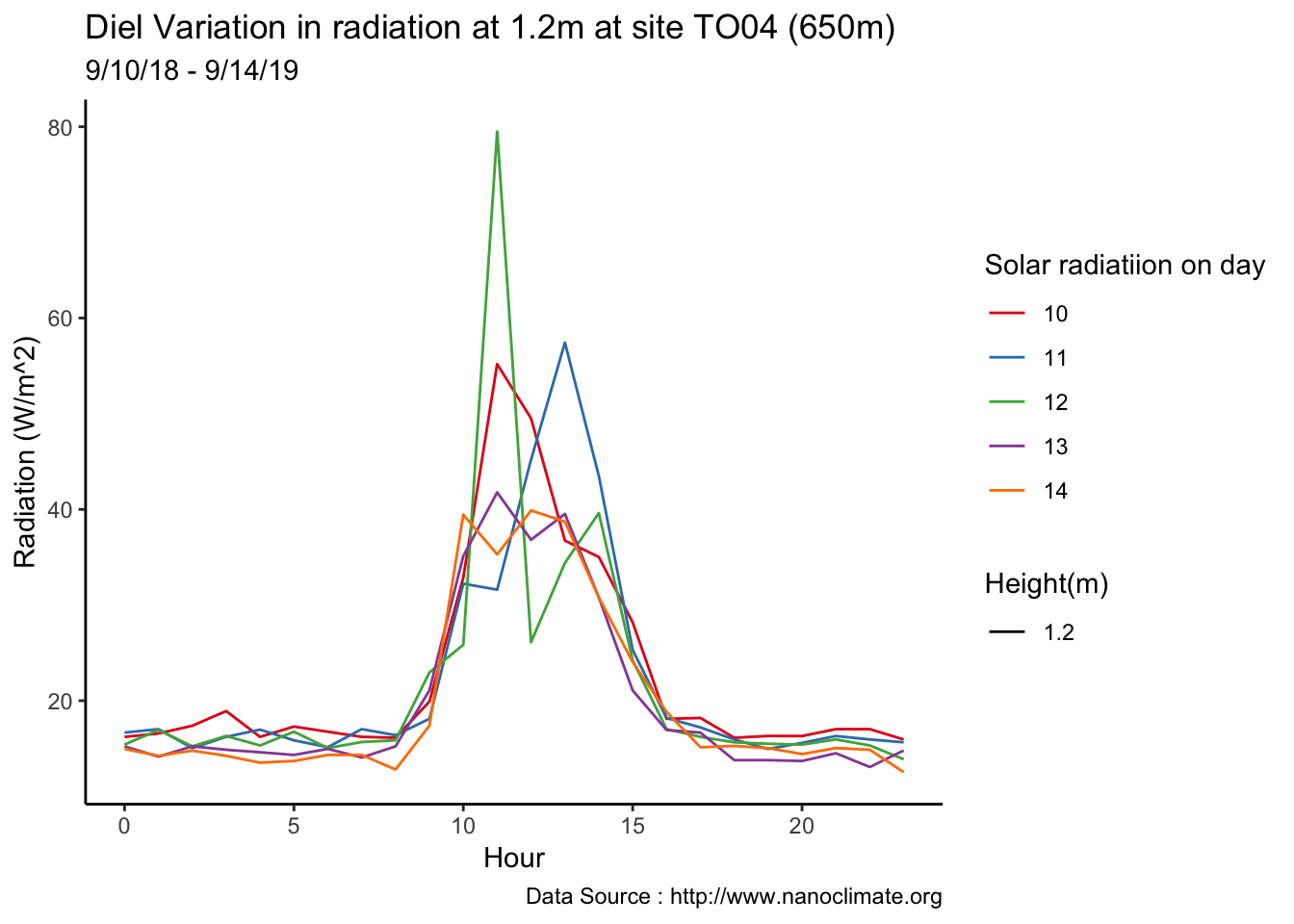
TO04
mclim_TO04_CN01_2018 %>% filter (!is.na(mclim_TO04_CN01_2018$minute) & month %in% c(9) ) %>%
filter( day > 9 & day < 15) %>%
mutate(solrf = ((solar-39) * 1.8) + ((25 -temp1) * .0012)) %>%
group_by(month,day,hr) %>%
add_count(wt=3) %>%
summarise(m1= mean(solrf)) %>%
group_by(day,hr) %>%
ggplot() +
geom_line(aes(hr,m1,group=day ,color=as.factor(day),linetype = '1.2'),se=F)+
scale_colour_manual("Solar radiatiion on day", breaks = c("10","11", "12","13","14"), values = brewer.pal(5, "Set1")) +
scale_linetype_manual("Height(m)",values=c("1.2"=1)) +
theme_classic() + ggtitle("Diel Variation in radiation at 1.2m at site TO04 (650m)") + xlab("Hour") +
ylab("Radiation (W/m^2)") + labs(colour = "Hour",
subtitle="9/10/18 - 9/14/19",caption="Data Source : http://www.nanoclimate.org") 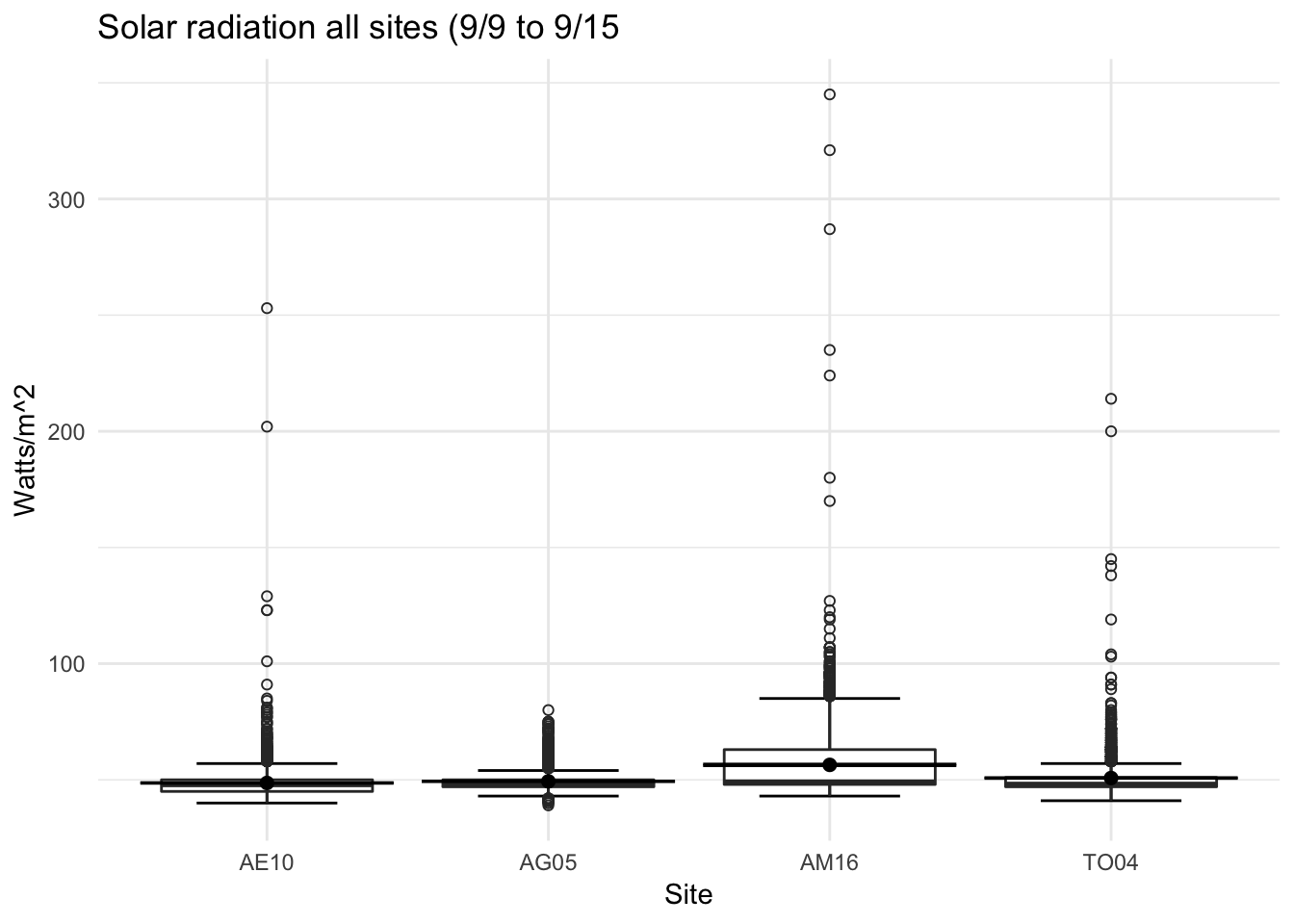
Box plot of all the stations
Does all the sites read the same solar radiation load ? Not really,
mclim_TO04_CN01_2018_wrk <- mclim_TO04_CN01_2018
mclim_TO04_CN01_2018_wrk$site <- 'TO04'
mclim_AM16_CN01_2018_wrk <- mclim_AM16_CN01_2018
mclim_AM16_CN01_2018_wrk$site <- 'AM16'
mclim_AE10_CN01_2018_wrk <- mclim_AE10_CN01_2018 %>% dplyr::select (-c(segment))
mclim_AE10_CN01_2018_wrk$site <- 'AE10'
mclim_AG05_CN01_2018_wrk <- mclim_AG05_CN01_2018
mclim_AG05_CN01_2018_wrk$site <- 'AG05'
mclim_CN01_2018_wrk<- rbind(mclim_TO04_CN01_2018_wrk,
mclim_AM16_CN01_2018_wrk,
mclim_AE10_CN01_2018_wrk,
mclim_AG05_CN01_2018_wrk
)
mclim_CN01_2018_wrk %>% dplyr::filter(solar < 750) %>%
filter (month %in% c(9) ) %>%
filter( day > 9 & day < 15) %>%
ggplot( aes(as.factor(site), solar))+
stat_boxplot( aes(as.factor(site), solar),
geom='errorbar', linetype=1, width=0.5)+ #whiskers
geom_boxplot( aes(as.factor(site), solar),outlier.shape=1) +
stat_summary(fun.y=mean, geom="point", size=2) +
stat_summary(fun.data = mean_se, geom = "errorbar") +
theme_minimal() +
ylab("Watts/m^2") + xlab("Site") +ggtitle("Solar radiation all sites (9/9 to 9/15") 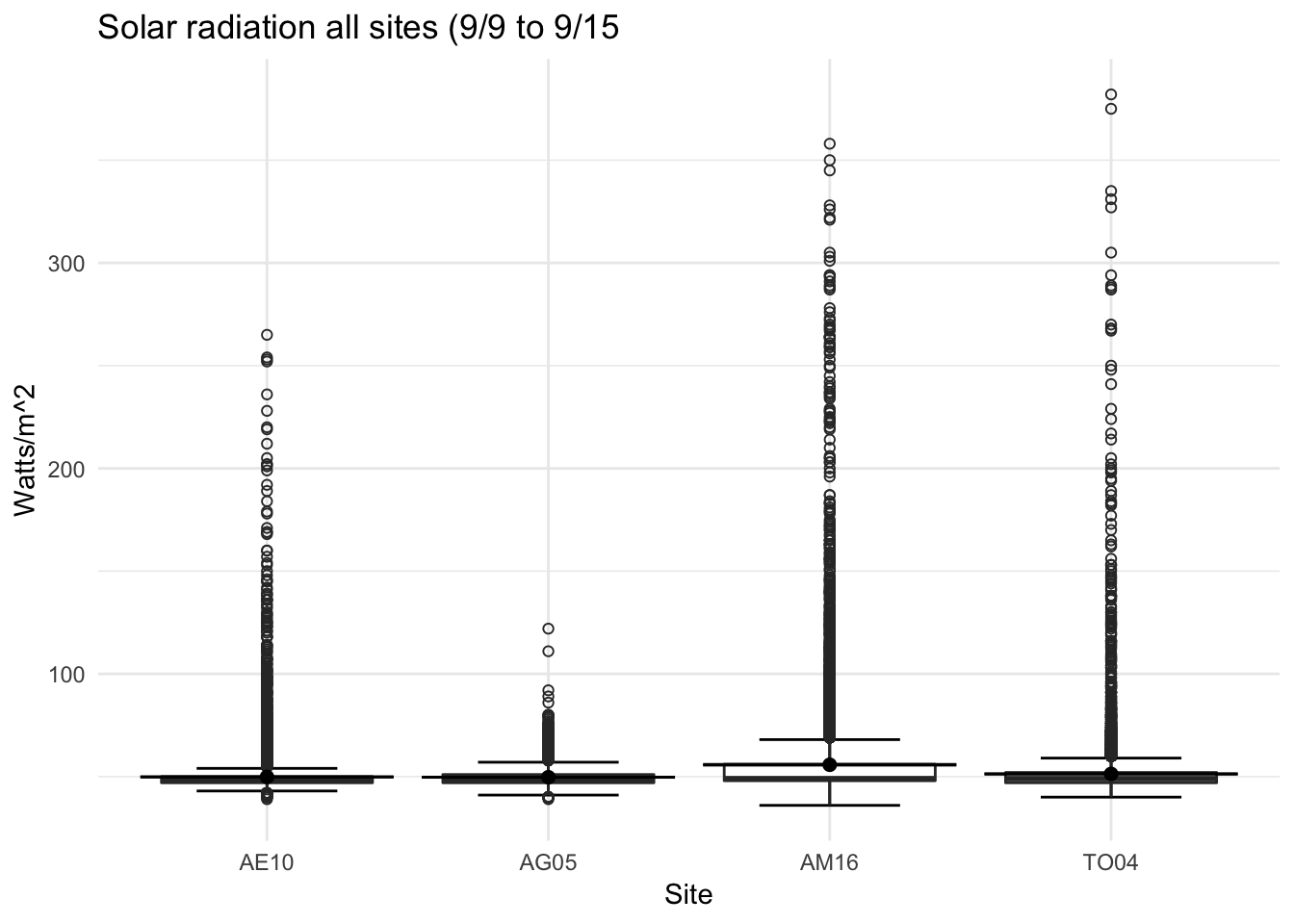
For the entire duration
mclim_CN01_2018_wrk %>% dplyr::filter(solar < 750) %>%
ggplot( aes(as.factor(site), solar))+
stat_boxplot( aes(as.factor(site), solar),
geom='errorbar', linetype=1, width=0.5)+ #whiskers
geom_boxplot( aes(as.factor(site), solar),outlier.shape=1) +
stat_summary(fun.y=mean, geom="point", size=2) +
stat_summary(fun.data = mean_se, geom = "errorbar") +
theme_minimal() +
ylab("Watts/m^2") + xlab("Site") +ggtitle("Solar radiation all sites (9/9 to 9/15") 
wind
mclim_CN01_2018_wrk %>% dplyr::filter(solar < 750) %>%
filter (month %in% c(9) ) %>%
filter( day > 9 & day < 15) %>%
ggplot( aes(as.factor(site), windspeed4))+
stat_boxplot( aes(as.factor(site), windspeed4),
geom='errorbar', linetype=1, width=0.5)+ #whiskers
geom_boxplot( aes(as.factor(site), windspeed4),outlier.shape=1) +
stat_summary(fun.y=mean, geom="point", size=2) +
stat_summary(fun.data = mean_se, geom = "errorbar") +
theme_minimal() +
ylab("km/h") + xlab("Site") +ggtitle("Wind all sites (9/9 to 9/15) - 0.3") 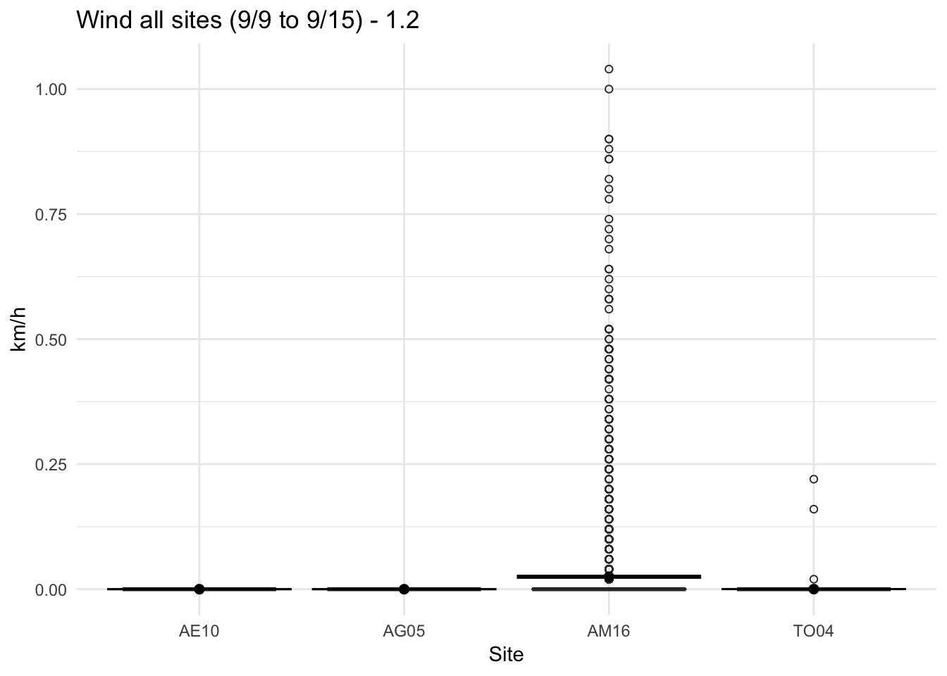
mclim_CN01_2018_wrk %>% dplyr::filter(solar < 750) %>%
filter (month %in% c(9) ) %>%
filter( day > 9 & day < 15) %>%
ggplot( aes(as.factor(site), windspeed1))+
stat_boxplot( aes(as.factor(site), windspeed1),
geom='errorbar', linetype=1, width=0.5)+ #whiskers
geom_boxplot( aes(as.factor(site), windspeed1),outlier.shape=1) +
stat_summary(fun.y=mean, geom="point", size=2) +
stat_summary(fun.data = mean_se, geom = "errorbar") +
theme_minimal() +
ylab("km/h") + xlab("Site") +ggtitle("Wind all sites (9/9 to 9/15) - 1.2") 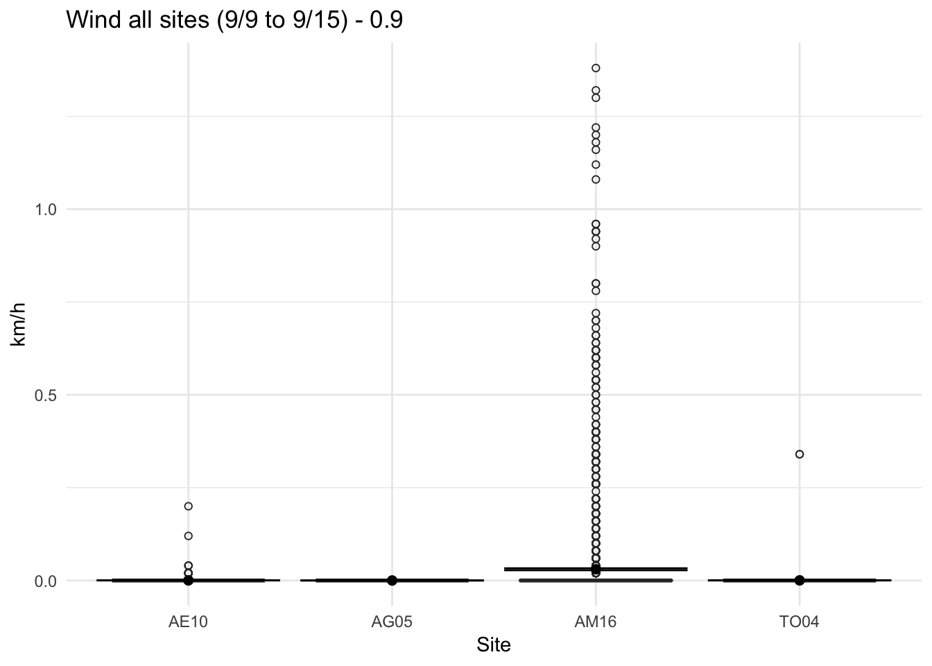
mclim_CN01_2018_wrk %>% dplyr::filter(solar < 750) %>%
filter (month %in% c(9) ) %>%
filter( day > 9 & day < 15) %>%
ggplot( aes(as.factor(site), windspeed2))+
stat_boxplot( aes(as.factor(site), windspeed2),
geom='errorbar', linetype=1, width=0.5)+ #whiskers
geom_boxplot( aes(as.factor(site), windspeed2),outlier.shape=1) +
stat_summary(fun.y=mean, geom="point", size=2) +
stat_summary(fun.data = mean_se, geom = "errorbar") +
theme_minimal() +
ylab("km/h") + xlab("Site") +ggtitle("Wind all sites (9/9 to 9/15) - 0.9") 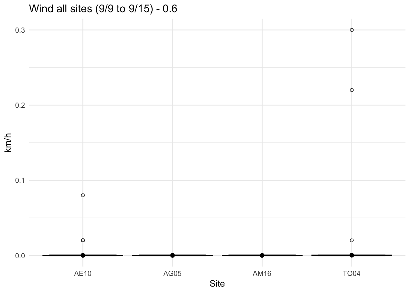
mclim_CN01_2018_wrk %>% dplyr::filter(solar < 750) %>%
filter (month %in% c(9) ) %>%
filter( day > 9 & day < 15) %>%
ggplot( aes(as.factor(site), windspeed3))+
stat_boxplot( aes(as.factor(site), windspeed3),
geom='errorbar', linetype=1, width=0.5)+ #whiskers
geom_boxplot( aes(as.factor(site), windspeed3),outlier.shape=1) +
stat_summary(fun.y=mean, geom="point", size=2) +
stat_summary(fun.data = mean_se, geom = "errorbar") +
theme_minimal() +
ylab("km/h") + xlab("Site") +ggtitle("Wind all sites (9/9 to 9/15) - 0.6") 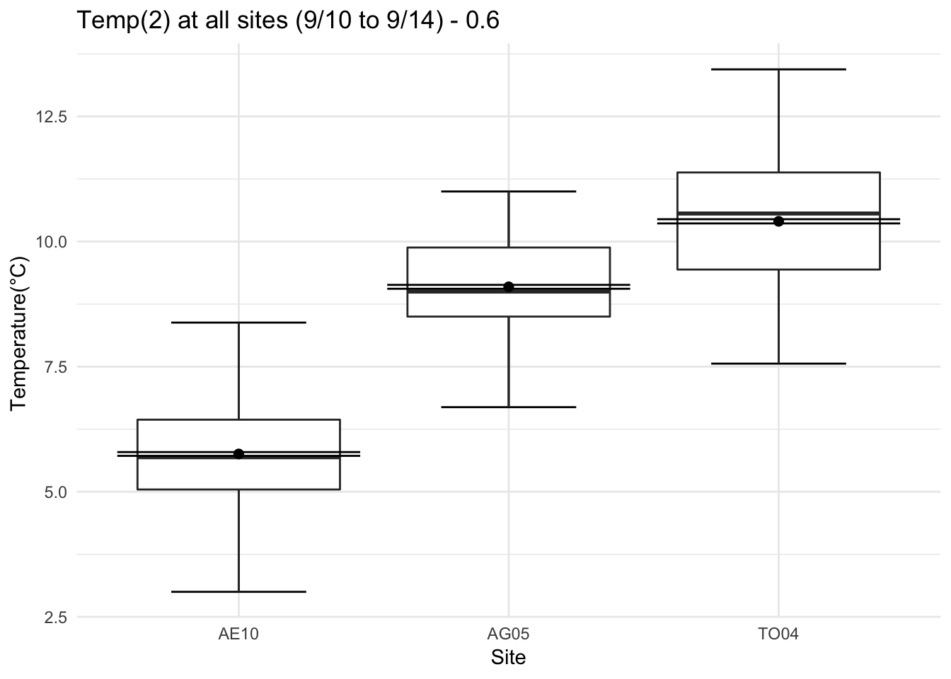
Temperature
Day time inversion ?
mclim_CN01_2018_wrk %>% dplyr::filter(temp2 >0 ) %>%
filter (month %in% c(9) ) %>%
filter( day > 9 & day < 15) %>%
filter(hr %in% c(8:15)) %>%
ggplot( aes(as.factor(site), temp2))+
stat_boxplot( aes(as.factor(site), temp2),
geom='errorbar', linetype=1, width=0.5)+ #whiskers
geom_boxplot( aes(as.factor(site), temp2),outlier.shape=1) +
stat_summary(fun.y=mean, geom="point", size=2) +
stat_summary(fun.data = mean_se, geom = "errorbar") +
theme_minimal() +
ylab("Temperature(°C) ") + xlab("Site") +ggtitle("Temp(2) at all sites (9/10 to 9/14) - 0.6") 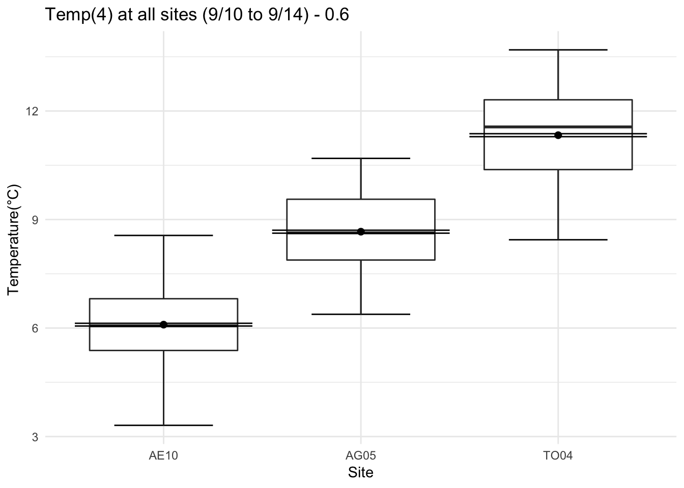
mclim_CN01_2018_wrk %>% dplyr::filter(temp4 >0 ) %>%
filter (month %in% c(9) ) %>%
filter( day > 9 & day < 15) %>%
filter(hr %in% c(8:15)) %>%
ggplot( aes(as.factor(site), temp4))+
stat_boxplot( aes(as.factor(site), temp4),
geom='errorbar', linetype=1, width=0.5)+ #whiskers
geom_boxplot( aes(as.factor(site), temp4),outlier.shape=1) +
stat_summary(fun.y=mean, geom="point", size=2) +
stat_summary(fun.data = mean_se, geom = "errorbar") +
theme_minimal() +
ylab("Temperature(°C) ") + xlab("Site") +ggtitle("Temp(4) at all sites (9/10 to 9/14) - 0.6") 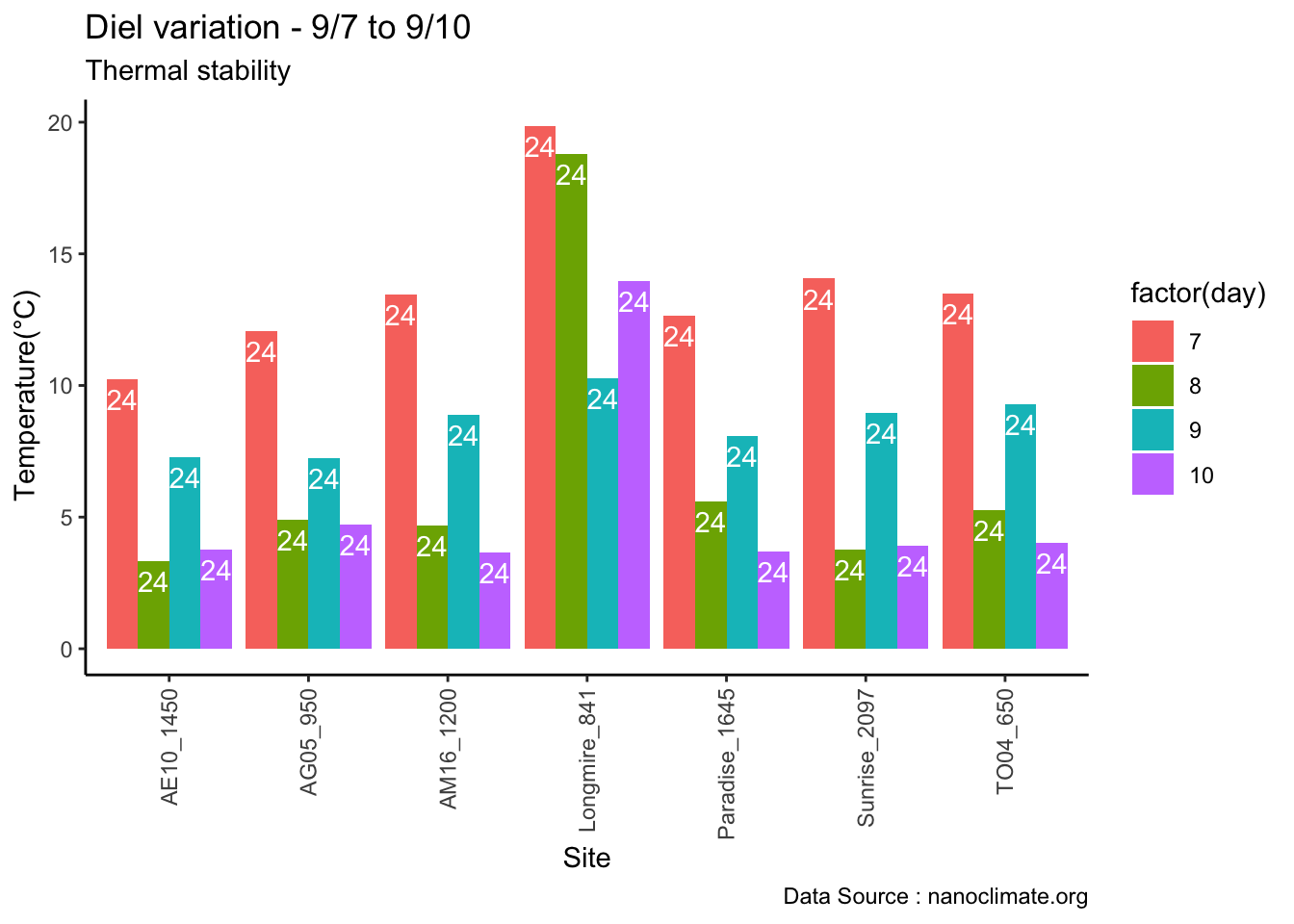
Checking stability
Way 1
combined_across_MM_and_PP_Long %>% dplyr::filter(day %in% c(7:10)) %>%
dplyr::group_by(site,day) %>% dplyr::summarise(dv=max(m1,na.rm = TRUE)- min(m1,na.rm = TRUE),no=n()) %>%
ggplot(aes(factor(site), dv, fill = factor(day))) +
geom_bar(stat = "identity", position = "dodge") +
geom_text(aes(label = round(no, 1)), position = position_dodge(0.9),
vjust = 1.5, color = "white") +
theme_classic() +
theme(axis.text.x = element_text(angle = 90, hjust = 1, vjust = .5)) +
labs(x="Site", y="Temperature(°C) ",subtitle="Thermal stability ", caption="Data Source : nanoclimate.org") +
ggtitle("Diel variation - 9/7 to 9/10")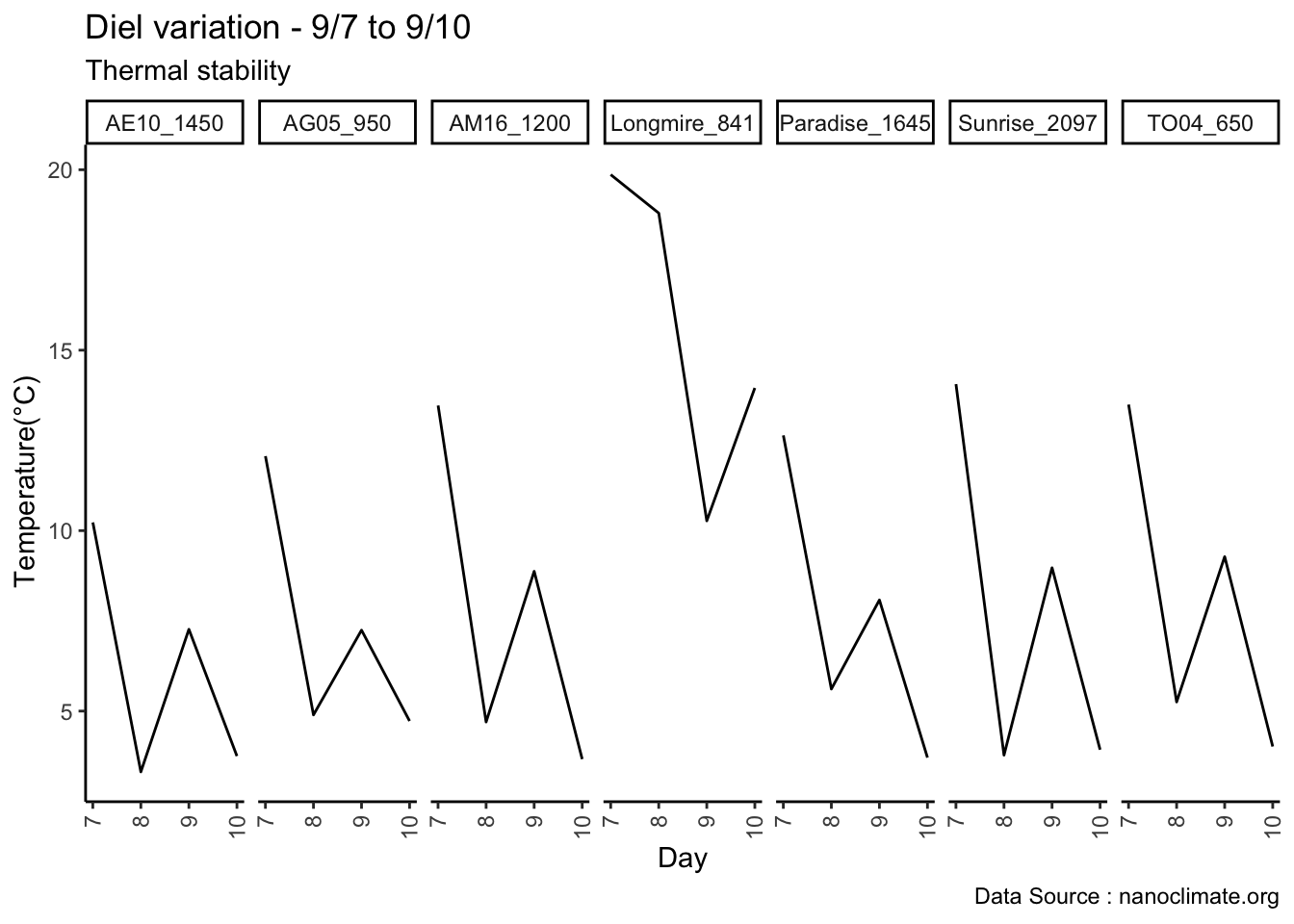
Way 2
combined_across_MM_and_PP_Long %>% dplyr::filter(day %in% c(7:10)) %>%
dplyr::group_by(site,day) %>% dplyr::summarise(dv=max(m1,na.rm = TRUE)- min(m1,na.rm = TRUE),no=n()) %>%
ggplot(aes(day, dv)) + geom_line() +
facet_grid(.~ site,scales = "free") +
theme_classic() +
theme(axis.text.x = element_text(angle = 90, hjust = 1, vjust = .5)) +
labs(x="Day", y="Temperature(°C) ",subtitle="Thermal stability ", caption="Data Source : nanoclimate.org") +
ggtitle("Diel variation - 9/7 to 9/10")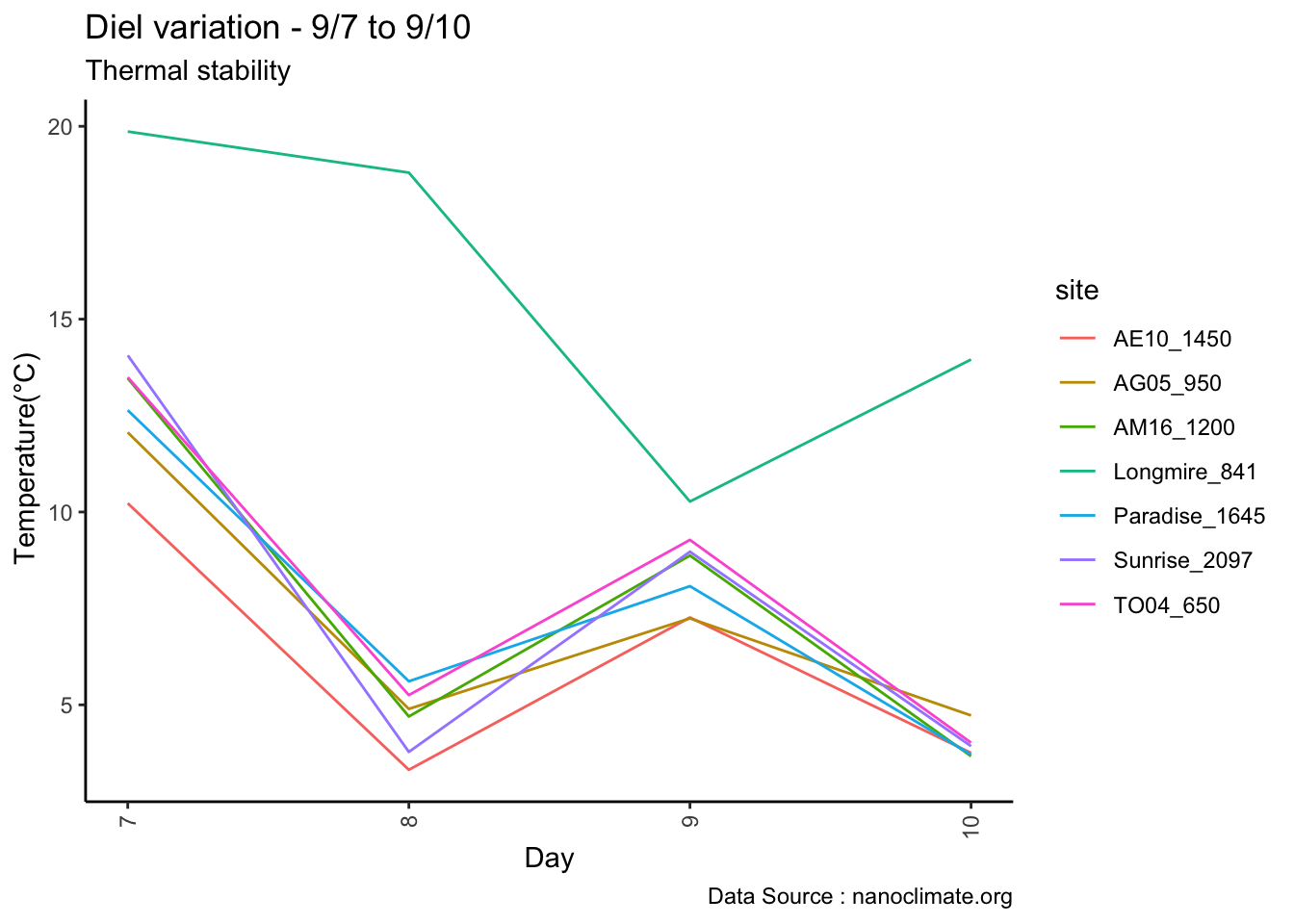
Way 3 (chosen)
combined_across_MM_and_PP_Long %>% dplyr::filter(day %in% c(7:10)) %>%
dplyr::group_by(site,day) %>% dplyr::summarise(dv=max(m1,na.rm = TRUE)- min(m1,na.rm = TRUE),no=n()) %>%
ggplot(aes(day, dv,color=site)) + geom_line() +
theme_classic() +
theme(axis.text.x = element_text(angle = 90, hjust = 1, vjust = .5)) +
labs(x="Day", y="Temperature(°C) ",subtitle="Thermal stability ", caption="Data Source : nanoclimate.org") +
ggtitle("Diel variation - 9/7 to 9/10")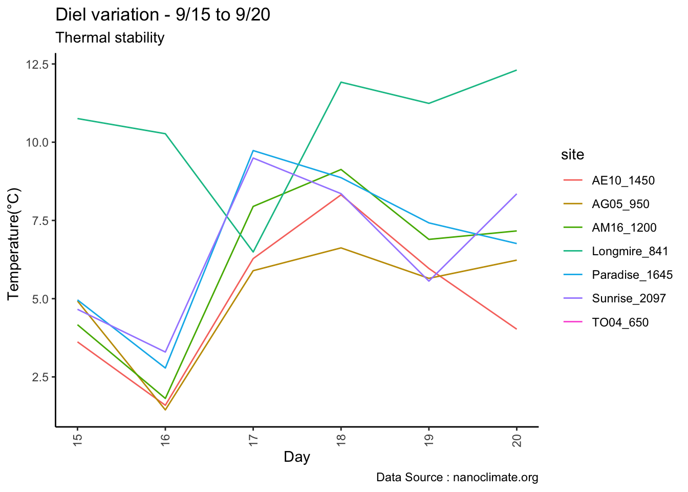
Differnt dates
combined_across_MM_and_PP_Long %>% dplyr::filter(day %in% c(15:20)) %>%
dplyr::group_by(site,day) %>% dplyr::summarise(dv=max(m1,na.rm = TRUE)- min(m1,na.rm = TRUE),no=n()) %>%
ggplot(aes(day, dv,color=site)) + geom_line() +
theme_classic() +
theme(axis.text.x = element_text(angle = 90, hjust = 1, vjust = .5)) +
labs(x="Day", y="Temperature(°C) ",subtitle="Thermal stability ", caption="Data Source : nanoclimate.org") +
ggtitle("Diel variation - 9/15 to 9/20")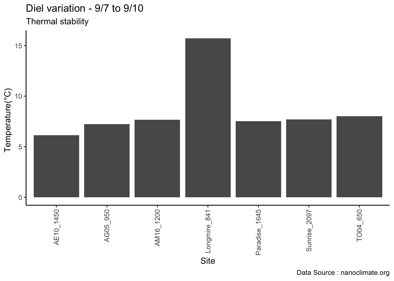
combined_across_MM_and_PP_Long %>% dplyr::filter(day %in% c(7:10)) %>%
dplyr::group_by(site,day) %>% dplyr::summarise(dv=max(m1,na.rm = TRUE)- min(m1,na.rm = TRUE),no=n()) %>% dplyr::group_by(site) %>% dplyr::summarise(dvt = mean(dv)) %>%
ggplot(aes(factor(site), dvt)) +
geom_bar(stat = "identity", position = "dodge") +
theme_classic() +
theme(axis.text.x = element_text(angle = 90, hjust = 1, vjust = .5)) +
labs(x="Site", y="Temperature(°C) ",subtitle="Thermal stability ", caption="Data Source : nanoclimate.org") +
ggtitle("Diel variation - 9/7 to 9/10")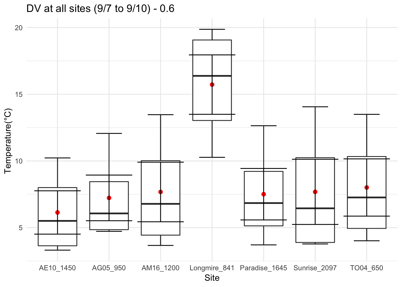
combined_across_MM_and_PP_Long %>% dplyr::filter(day %in% c(7:10)) %>%
dplyr::group_by(site,day) %>% dplyr::summarise(dv=max(m1,na.rm = TRUE)- min(m1,na.rm = TRUE),no=n()) %>%
ggplot( aes(as.factor(site), dv))+
stat_boxplot( aes(as.factor(site), dv),
geom='errorbar', linetype=1, width=0.5)+ #whiskers
geom_boxplot( aes(as.factor(site), dv),outlier.shape=1) +
stat_summary(fun.y=mean, geom="point", size=2,color="red") +
stat_summary(fun.data = mean_se, geom = "errorbar") +
theme_minimal() +
ylab("Temperature(°C) ") + xlab("Site") +ggtitle("DV at all sites (9/7 to 9/10) - 0.6") 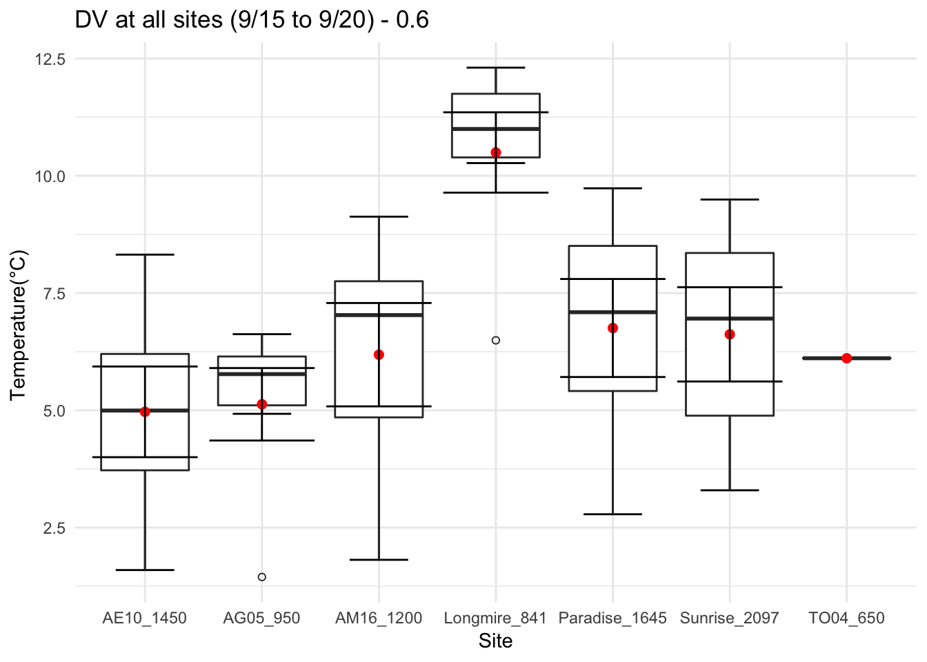
combined_across_MM_and_PP_Long %>% dplyr::filter(day %in% c(15:20)) %>%
dplyr::group_by(site,day) %>% dplyr::summarise(dv=max(m1,na.rm = TRUE)- min(m1,na.rm = TRUE),no=n()) %>%
ggplot( aes(as.factor(site), dv))+
stat_boxplot( aes(as.factor(site), dv),
geom='errorbar', linetype=1, width=0.5)+ #whiskers
geom_boxplot( aes(as.factor(site), dv),outlier.shape=1) +
stat_summary(fun.y=mean, geom="point", size=2,color="red") +
stat_summary(fun.data = mean_se, geom = "errorbar") +
theme_minimal() +
ylab("Temperature(°C) ") + xlab("Site") +ggtitle("DV at all sites (9/15 to 9/20) - 0.6") 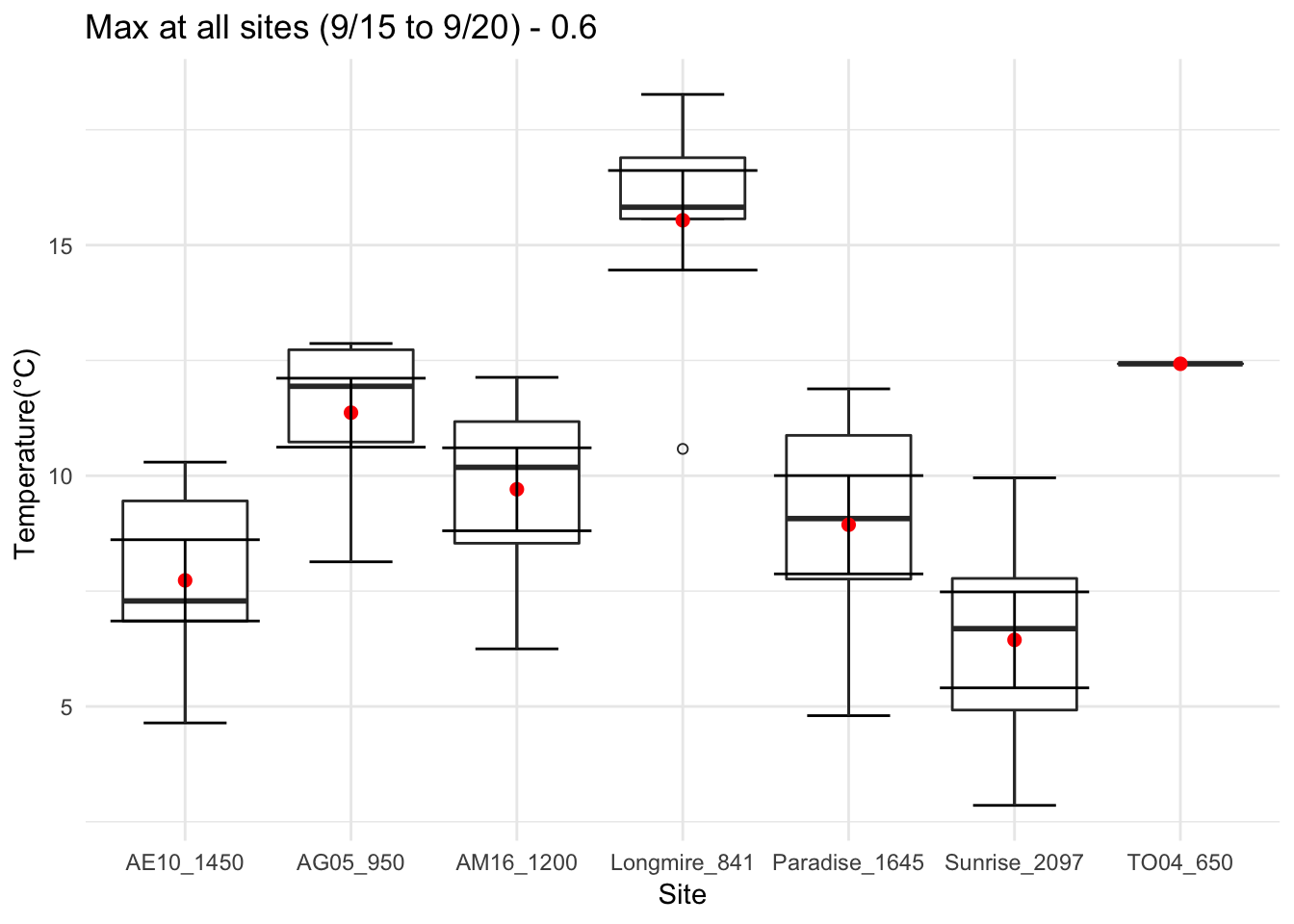
Existing understanding ( Max and mean temp)
combined_across_MM_and_PP_Long %>% dplyr::filter(day %in% c(15:20)) %>%
dplyr::group_by(site,day) %>% dplyr::summarise(maxt=max(m1,na.rm = TRUE),mint= min(m1,na.rm = TRUE),no=n()) %>%
ggplot( aes(as.factor(site), maxt))+
stat_boxplot( aes(as.factor(site), maxt),
geom='errorbar', linetype=1, width=0.5)+ #whiskers
geom_boxplot( aes(as.factor(site), maxt),outlier.shape=1) +
stat_summary(fun.y=mean, geom="point", size=2,color="red") +
stat_summary(fun.data = mean_se, geom = "errorbar") +
theme_minimal() +
ylab("Temperature(°C) ") + xlab("Site") +ggtitle("Max at all sites (9/15 to 9/20) - 0.6") 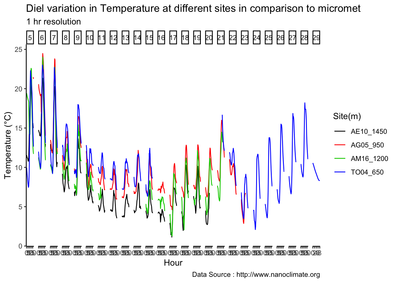 Data rep
combined_across_MM_and_PP_Long %>% filter (month %in% c(9) & !site %in% c('Longmire_841','Sunrise_2097','Paradise_1645') ) %>%
ggplot() +
geom_line(aes(hr,m1,color = site),se=F)+
facet_grid(. ~ day, scales = "free") +
scale_color_manual("Site(m)",values=c("AE10_1450"=1,"AG05_950"=2,"AM16_1200"=3,"TO04_650"=4,"Paradise_1645"=5,"Sunrise_2097"=6,"Longmire_841"=8)) +
theme_classic() + ggtitle("Diel variation in Temperature at different sites in comparison to micromet") + xlab("Hour") +
ylab("Temperature (°C)") + labs(colour = "Hour",
subtitle="1 hr resolution",caption="Data Source : http://www.nanoclimate.org") 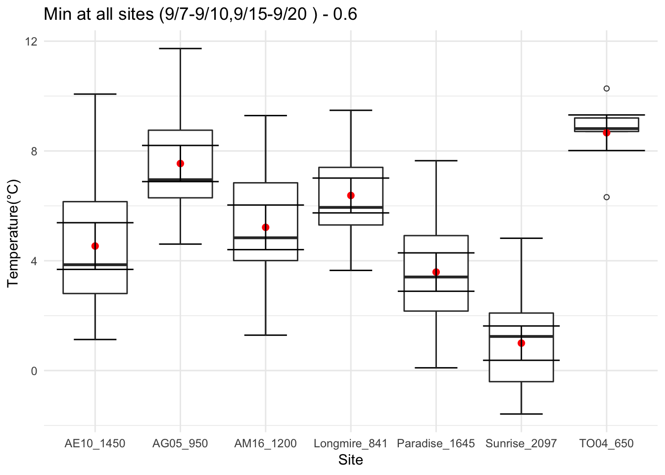 ## 2-25-2019
Existing understanding ( Min and mean temp)
## 2-25-2019
Existing understanding ( Min and mean temp)
combined_across_MM_and_PP_Long %>% dplyr::filter(day %in% c(15:20,c(7:10))) %>%
dplyr::group_by(site,day) %>% dplyr::summarise(meant=mean(m1,na.rm = TRUE),mint= min(m1,na.rm = TRUE),no=n()) %>%
ggplot( aes(as.factor(site), mint))+
stat_boxplot( aes(as.factor(site), mint),
geom='errorbar', linetype=1, width=0.5)+ #whiskers
geom_boxplot( aes(as.factor(site), mint),outlier.shape=1) +
stat_summary(fun.y=mean, geom="point", size=2,color="red") +
stat_summary(fun.data = mean_se, geom = "errorbar") +
theme_minimal() +
ylab("Temperature(°C) ") + xlab("Site") +ggtitle("Min at all sites (9/7-9/10,9/15-9/20 ) - 0.6") 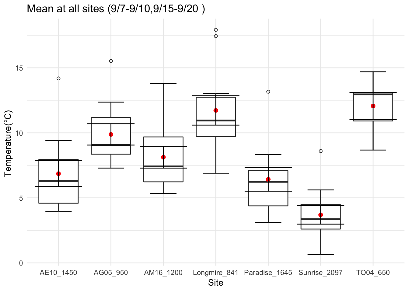
combined_across_MM_and_PP_Long %>% dplyr::filter(day %in% c(15:20,c(7:10))) %>%
dplyr::group_by(site,day) %>% dplyr::summarise(meant=mean(m1,na.rm = TRUE),mint= min(m1,na.rm = TRUE),no=n()) %>%
ggplot( aes(as.factor(site), meant))+
stat_boxplot( aes(as.factor(site), meant),
geom='errorbar', linetype=1, width=0.5)+ #whiskers
geom_boxplot( aes(as.factor(site), meant),outlier.shape=1) +
stat_summary(fun.y=mean, geom="point", size=2,color="red") +
stat_summary(fun.data = mean_se, geom = "errorbar") +
theme_minimal() +
ylab("Temperature(°C) ") + xlab("Site") +ggtitle("Mean at all sites (9/7-9/10,9/15-9/20 )") 
combined_across_MM_and_PP_Long %>% dplyr::filter(day %in% c(15:20,c(7:10))) %>%
dplyr::group_by(site,day) %>% dplyr::summarise(maxt=max(m1,na.rm = TRUE),mint= min(m1,na.rm = TRUE),no=n()) %>%
ggplot( aes(as.factor(site), maxt))+
stat_boxplot( aes(as.factor(site), maxt),
geom='errorbar', linetype=1, width=0.5)+ #whiskers
geom_boxplot( aes(as.factor(site), maxt),outlier.shape=1) +
stat_summary(fun.y=mean, geom="point", size=2,color="red") +
stat_summary(fun.data = mean_se, geom = "errorbar") +
theme_minimal() +
ylab("Temperature(°C) ") + xlab("Site") +ggtitle("Max at all sites (9/7-9/10,9/15-9/20 )") 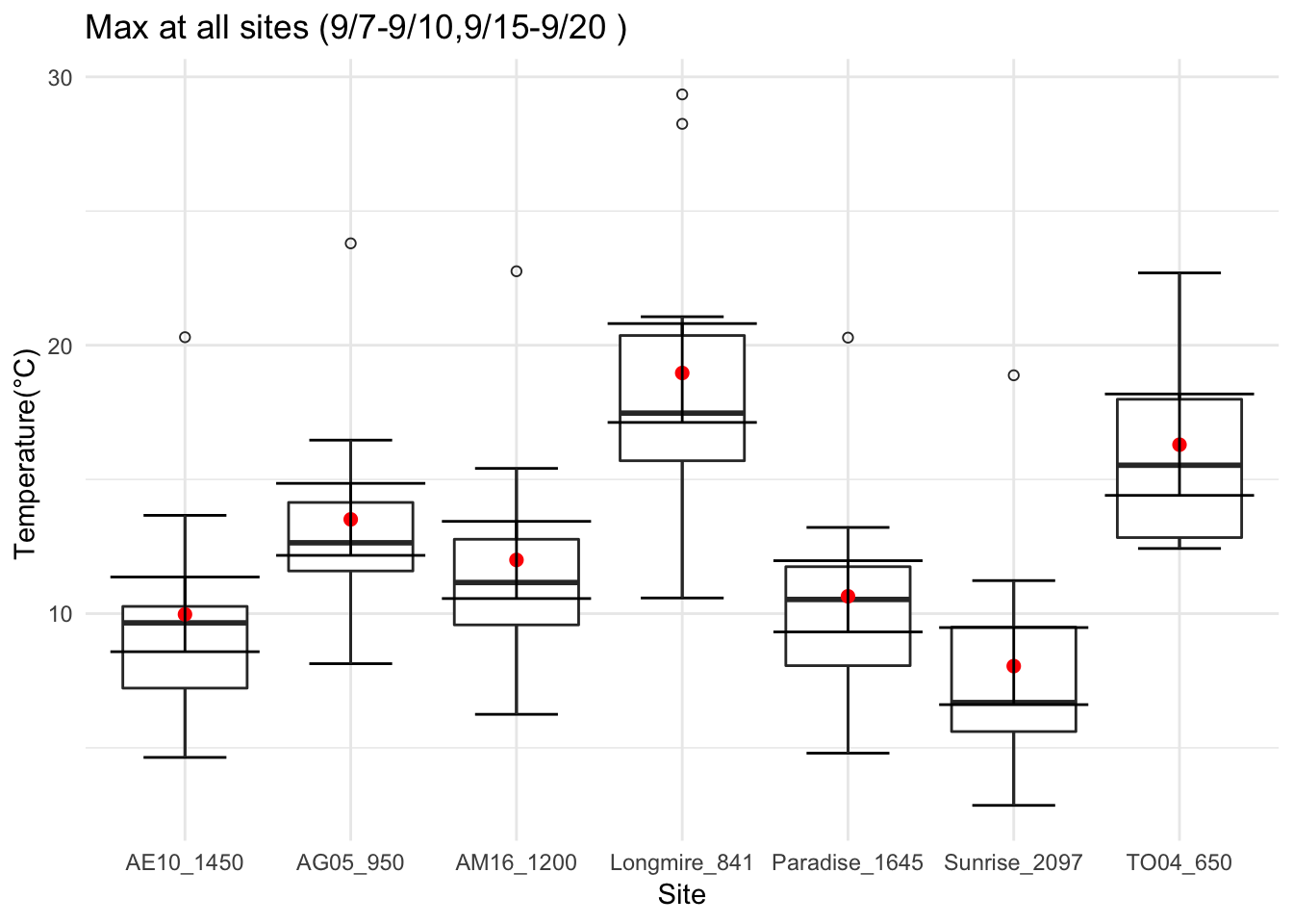
All three together
combined_across_MM_and_PP_Long %>% dplyr::filter(day %in% c(15:20,c(7:10))) %>%
dplyr::group_by(site,day) %>% dplyr::summarise(maxt=max(m1,na.rm = TRUE),mint= min(m1,na.rm = TRUE),meant= mean(m1,na.rm = TRUE),no=n()) %>%
ggplot( aes(as.factor(site), maxt))+
stat_boxplot( aes(as.factor(site), maxt),
geom='errorbar', linetype=1, width=0.5)+ #whiskers
geom_boxplot( aes(as.factor(site), maxt),outlier.shape=1) +
stat_summary(fun.y=mean, geom="point", size=2,color="red") +
stat_summary(fun.data = mean_se, geom = "errorbar") +
theme_minimal() +
ylab("Temperature(°C) ") + xlab("Site") +ggtitle("Max at all sites (9/7-9/10,9/15-9/20 )") 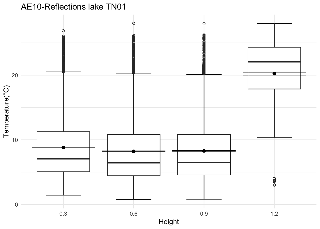
Height plots with temperature
AE10 - TN01
mclim_AE10_TN01_2018 %>% dplyr::filter(temp > -10) %>%
ggplot(aes(as.factor(height), temp))+
stat_boxplot( aes(as.factor(height), temp),
geom='errorbar', linetype=1, width=0.5)+ #whiskers
geom_boxplot( aes(as.factor(height), temp),outlier.shape=1) +
stat_summary(fun.y=mean, geom="point", size=2) +
stat_summary(fun.data = mean_se, geom = "errorbar") +
theme_minimal() +
ylab("Temperature(°C)") + xlab("Height") +ggtitle("AE10-Reflections lake TN01") 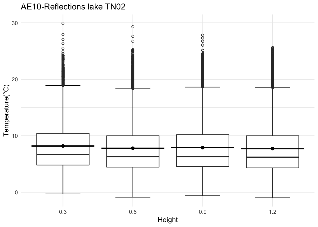
AE10 - TN02
mclim_AE10_TN02_2018 %>% dplyr::filter(temp > -10) %>%
ggplot(aes(as.factor(height), temp))+
stat_boxplot( aes(as.factor(height), temp),
geom='errorbar', linetype=1, width=0.5)+ #whiskers
geom_boxplot( aes(as.factor(height), temp),outlier.shape=1) +
stat_summary(fun.y=mean, geom="point", size=2) +
stat_summary(fun.data = mean_se, geom = "errorbar") +
theme_minimal() +
ylab("Temperature(°C)") + xlab("Height") +ggtitle("AE10-Reflections lake TN02") 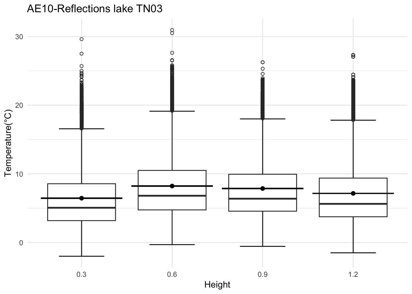
AE10 - TN03
mclim_AE10_TN03_2018 %>% dplyr::filter(temp > -10) %>%
ggplot(aes(as.factor(height), temp))+
stat_boxplot( aes(as.factor(height), temp),
geom='errorbar', linetype=1, width=0.5)+ #whiskers
geom_boxplot( aes(as.factor(height), temp),outlier.shape=1) +
stat_summary(fun.y=mean, geom="point", size=2) +
stat_summary(fun.data = mean_se, geom = "errorbar") +
theme_minimal() +
ylab("Temperature(°C)") + xlab("Height") +ggtitle("AE10-Reflections lake TN03") 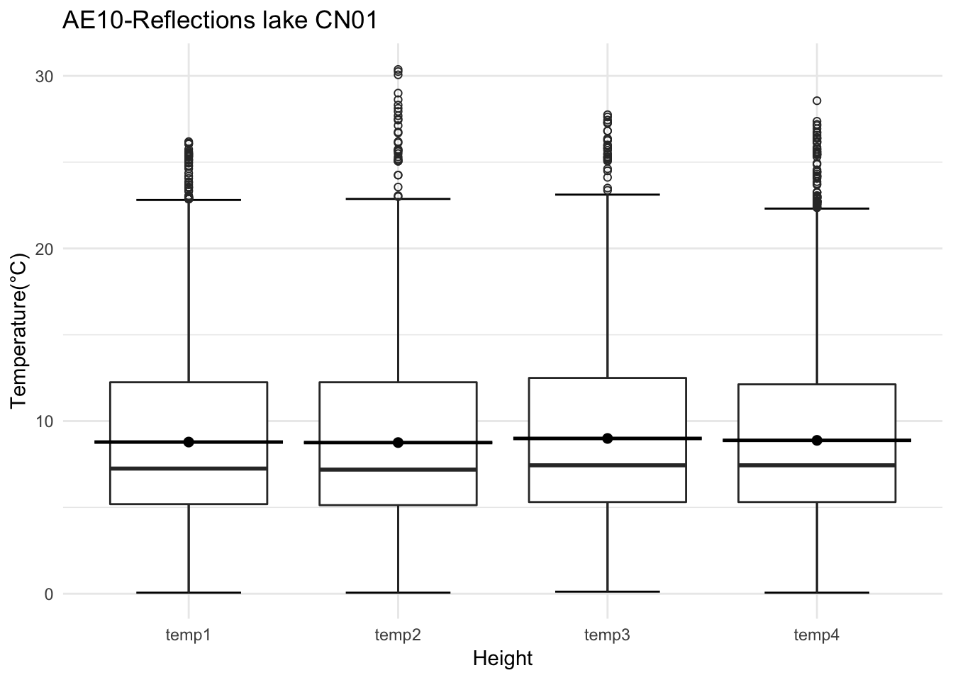
AE10 CN01
mclim_AE10_CN01_2018 %>% dplyr::select(time, temp1,temp2,temp3,temp4) %>%
dplyr::filter(temp1 >0 & temp2 >0 & temp3 >0 & temp4 > 0 ) %>%
dplyr::filter(temp1 <50 & temp2 <50 & temp3 <50 & temp4 < 50 ) %>%
gather(variable, value,-time) %>%
ggplot( aes(as.factor(variable), value))+
stat_boxplot( aes(as.factor(variable), value),
geom='errorbar', linetype=1, width=0.5)+ #whiskers
geom_boxplot( aes(as.factor(variable), value),outlier.shape=1) +
stat_summary(fun.y=mean, geom="point", size=2) +
stat_summary(fun.data = mean_se, geom = "errorbar") +
theme_minimal() +
ylab("Temperature(°C)") + xlab("Height") +ggtitle("AE10-Reflections lake CN01") 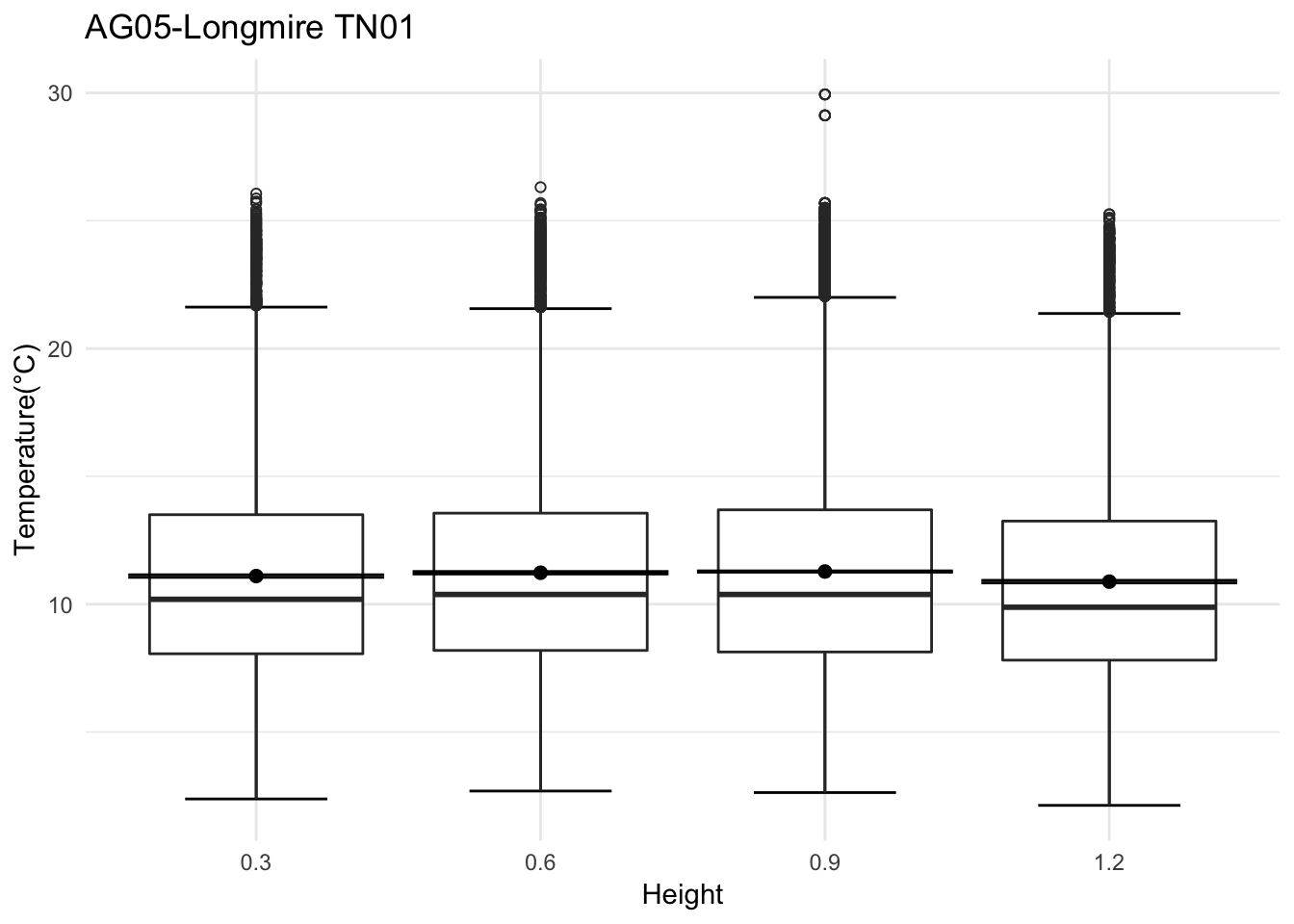 AG05
AG05
TN01
mclim_AG05_TN01_2018 %>% dplyr::filter(temp > -10) %>%
ggplot(aes(as.factor(height), temp))+
stat_boxplot( aes(as.factor(height), temp),
geom='errorbar', linetype=1, width=0.5)+ #whiskers
geom_boxplot( aes(as.factor(height), temp),outlier.shape=1) +
stat_summary(fun.y=mean, geom="point", size=2) +
stat_summary(fun.data = mean_se, geom = "errorbar") +
theme_minimal() +
ylab("Temperature(°C)") + xlab("Height") +ggtitle("AG05-Longmire TN01") 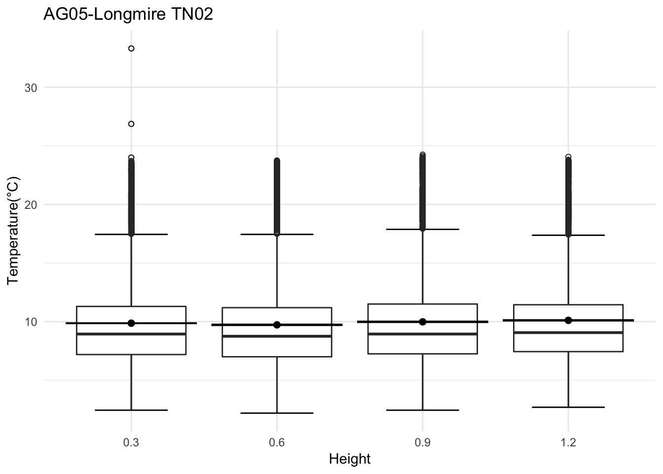 AG05 TN02
mclim_AG05_TN02_2018 %>% dplyr::filter(temp > -10) %>%
ggplot(aes(as.factor(height), temp))+
stat_boxplot( aes(as.factor(height), temp),
geom='errorbar', linetype=1, width=0.5)+ #whiskers
geom_boxplot( aes(as.factor(height), temp),outlier.shape=1) +
stat_summary(fun.y=mean, geom="point", size=2) +
stat_summary(fun.data = mean_se, geom = "errorbar") +
theme_minimal() +
ylab("Temperature(°C)") + xlab("Height") +ggtitle("AG05-Longmire TN02") 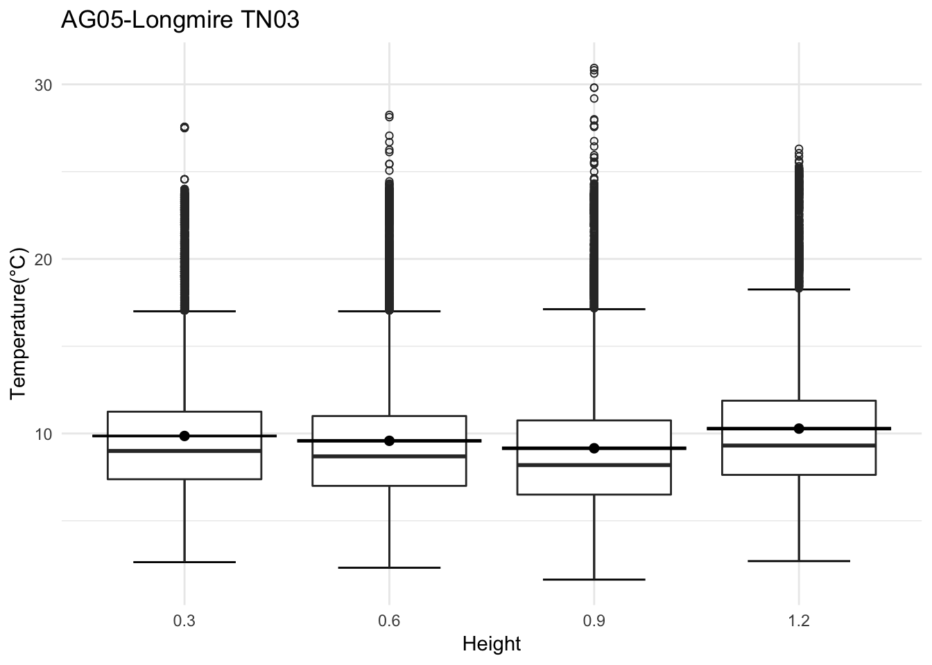
AG05 - TN03
mclim_AG05_TN03_2018 %>% dplyr::filter(temp > -10) %>%
ggplot(aes(as.factor(height), temp))+
stat_boxplot( aes(as.factor(height), temp),
geom='errorbar', linetype=1, width=0.5)+ #whiskers
geom_boxplot( aes(as.factor(height), temp),outlier.shape=1) +
stat_summary(fun.y=mean, geom="point", size=2) +
stat_summary(fun.data = mean_se, geom = "errorbar") +
theme_minimal() +
ylab("Temperature(°C)") + xlab("Height") +ggtitle("AG05-Longmire TN03") 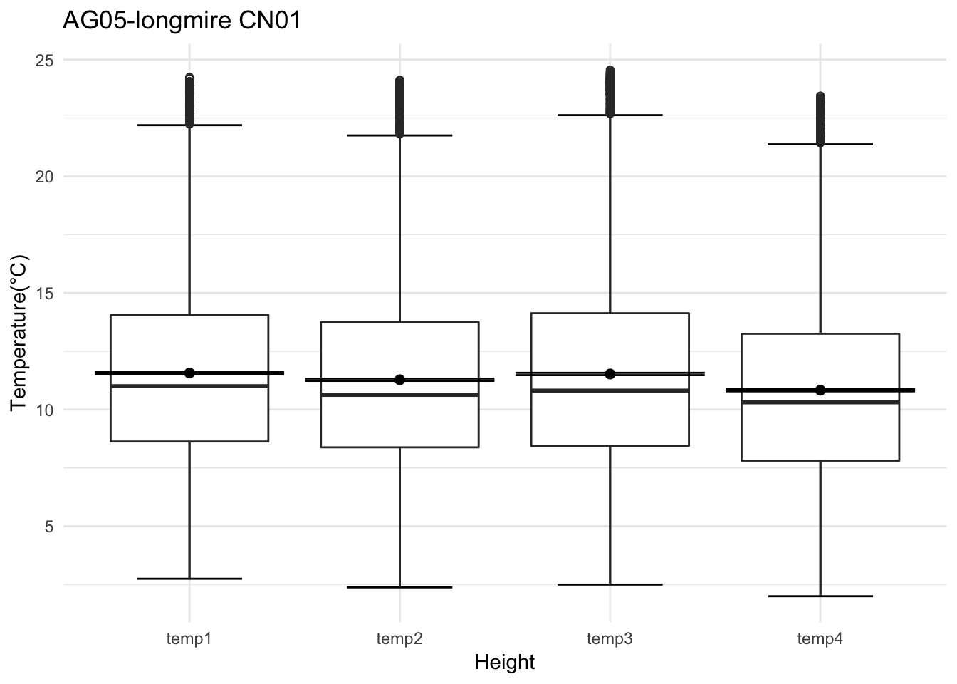
AG05 CN01
mclim_AG05_CN01_2018 %>% dplyr::select(time, temp1,temp2,temp3,temp4) %>%
dplyr::filter(temp1 >0 & temp2 >0 & temp3 >0 & temp4 > 0 ) %>%
dplyr::filter(temp1 <50 & temp2 <50 & temp3 <50 & temp4 < 50 ) %>%
gather(variable, value,-time) %>%
ggplot( aes(as.factor(variable), value))+
stat_boxplot( aes(as.factor(variable), value),
geom='errorbar', linetype=1, width=0.5)+ #whiskers
geom_boxplot( aes(as.factor(variable), value),outlier.shape=1) +
stat_summary(fun.y=mean, geom="point", size=2) +
stat_summary(fun.data = mean_se, geom = "errorbar") +
theme_minimal() +
ylab("Temperature(°C)") + xlab("Height") +ggtitle("AG05-longmire CN01") 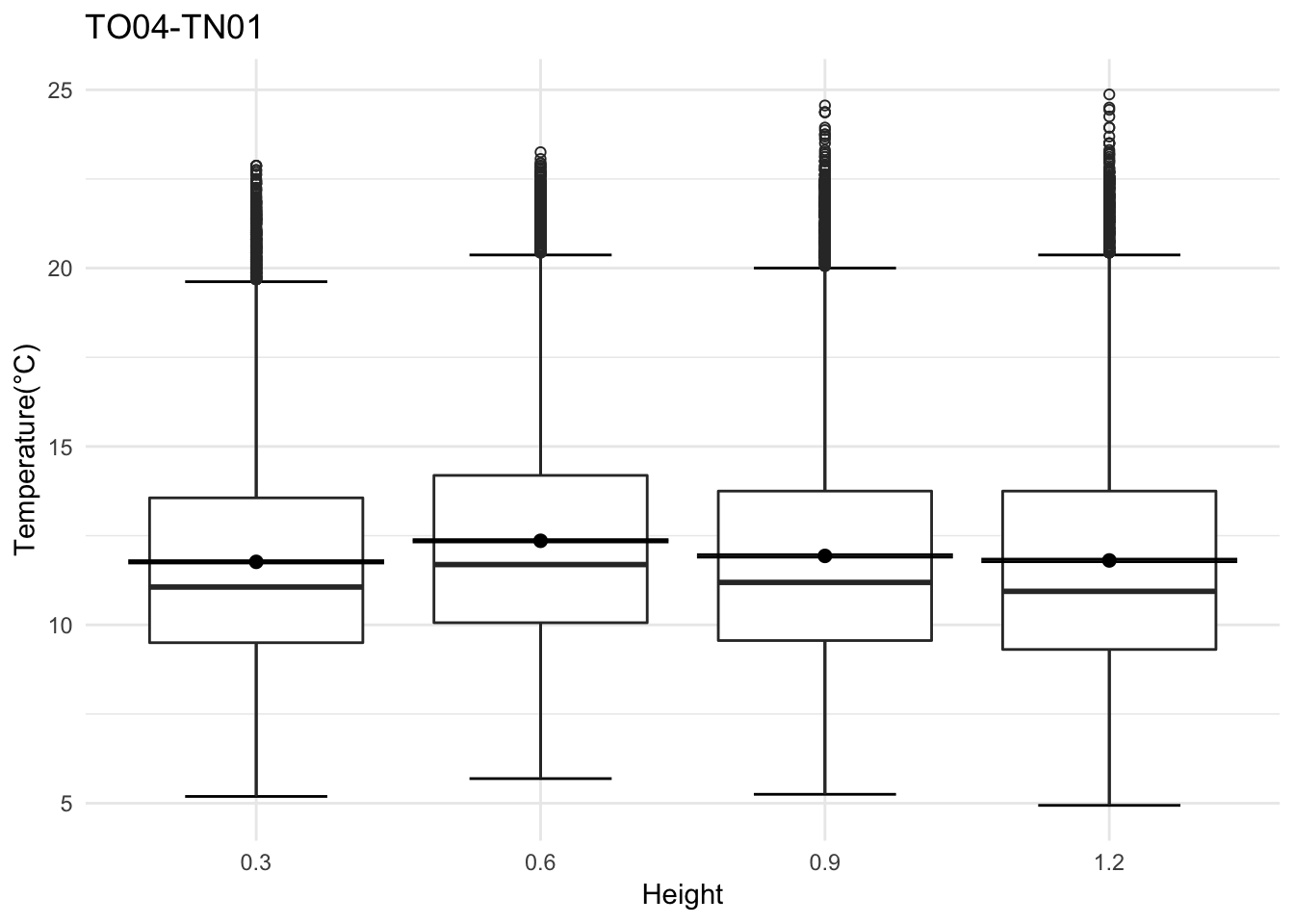
TO04 TN01
mclim_TO04_TN01_2018 %>% dplyr::filter(temp > -10) %>%
ggplot(aes(as.factor(height), temp))+
stat_boxplot( aes(as.factor(height), temp),
geom='errorbar', linetype=1, width=0.5)+ #whiskers
geom_boxplot( aes(as.factor(height), temp),outlier.shape=1) +
stat_summary(fun.y=mean, geom="point", size=2) +
stat_summary(fun.data = mean_se, geom = "errorbar") +
theme_minimal() +
ylab("Temperature(°C)") + xlab("Height") +ggtitle("TO04-TN01") 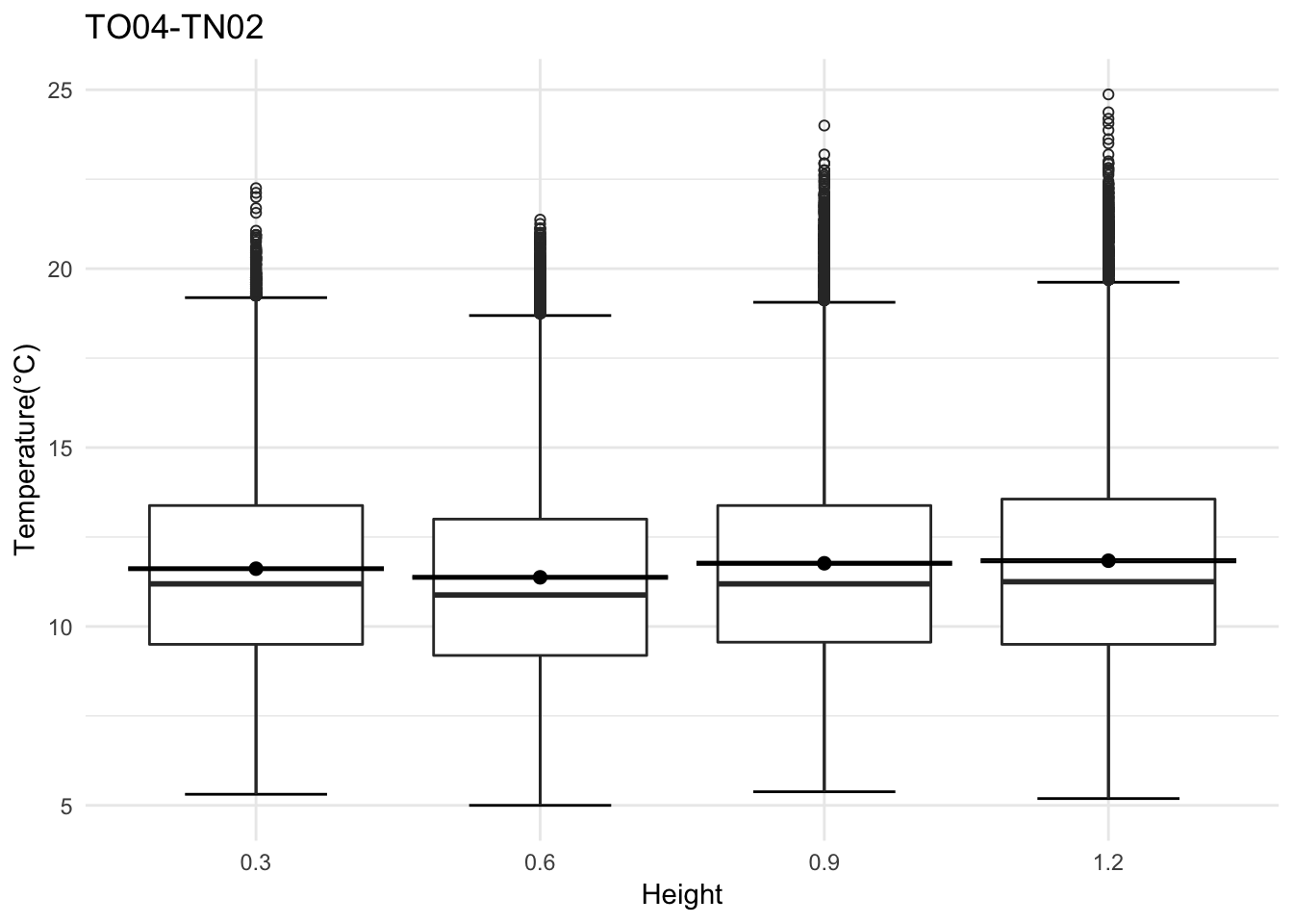
mclim_TO04_TN02_2018 %>% dplyr::filter(temp > -10 & height >0) %>%
ggplot(aes(as.factor(height), temp))+
stat_boxplot( aes(as.factor(height), temp),
geom='errorbar', linetype=1, width=0.5)+ #whiskers
geom_boxplot( aes(as.factor(height), temp),outlier.shape=1) +
stat_summary(fun.y=mean, geom="point", size=2) +
stat_summary(fun.data = mean_se, geom = "errorbar") +
theme_minimal() +
ylab("Temperature(°C)") + xlab("Height") +ggtitle("TO04-TN02") 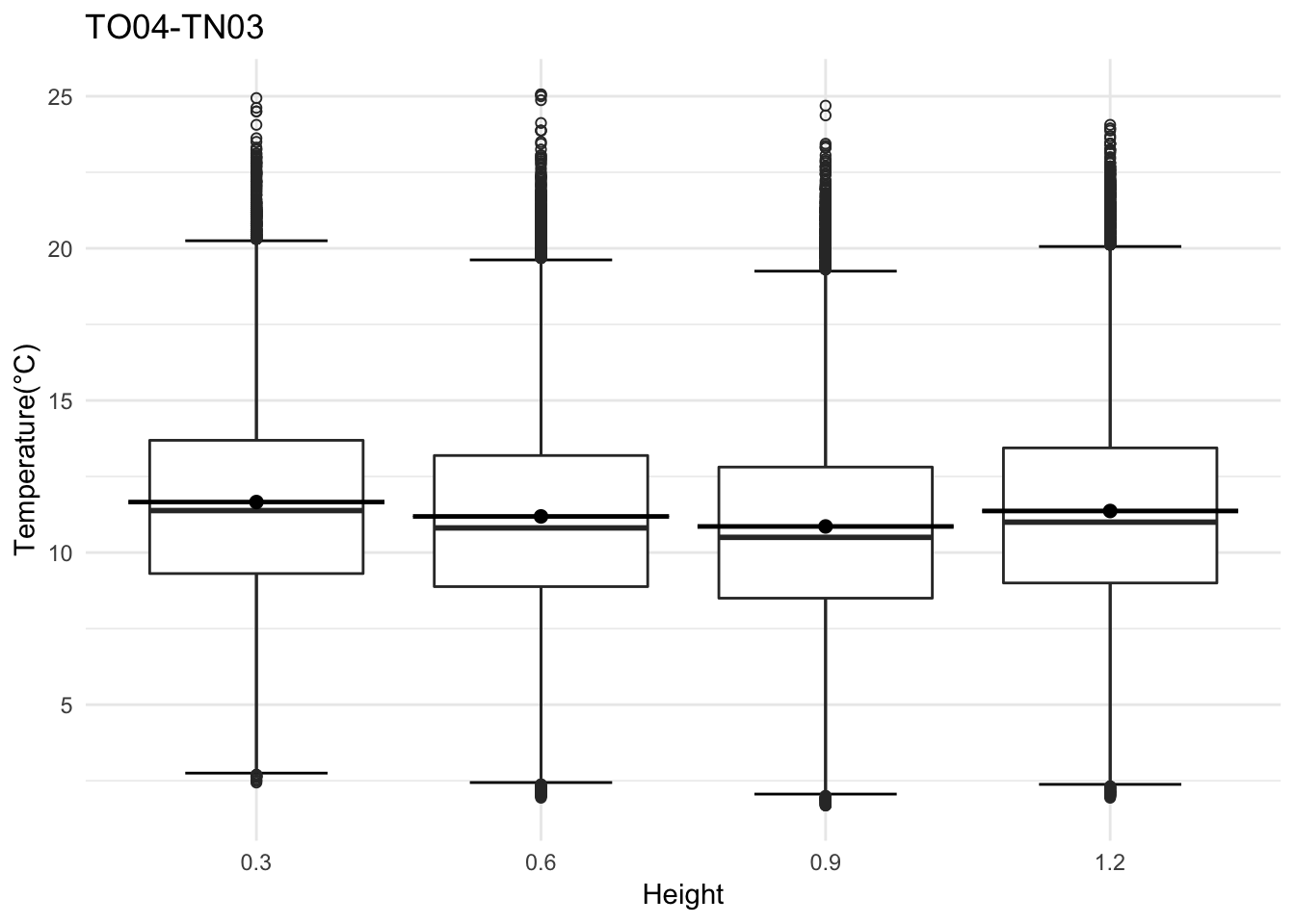
mclim_TO04_TN03_2018 %>% dplyr::filter(temp > -10) %>%
ggplot(aes(as.factor(height), temp))+
stat_boxplot( aes(as.factor(height), temp),
geom='errorbar', linetype=1, width=0.5)+ #whiskers
geom_boxplot( aes(as.factor(height), temp),outlier.shape=1) +
stat_summary(fun.y=mean, geom="point", size=2) +
stat_summary(fun.data = mean_se, geom = "errorbar") +
theme_minimal() +
ylab("Temperature(°C)") + xlab("Height") +ggtitle("TO04-TN03") 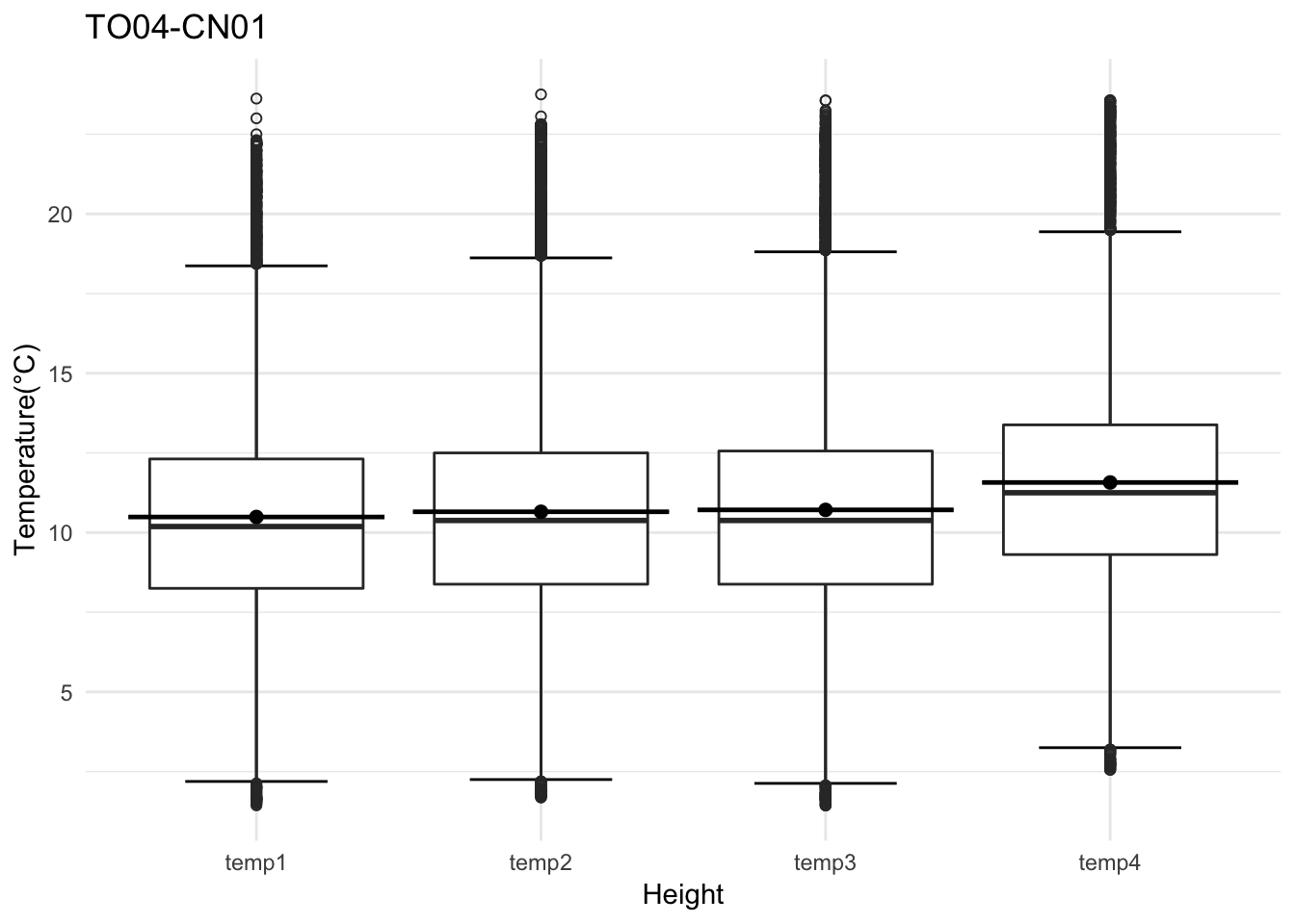
CN01
mclim_TO04_CN01_2018 %>% dplyr::select(time, temp1,temp2,temp3,temp4) %>%
dplyr::filter(temp1 >0 & temp2 >0 & temp3 >0 & temp4 > 0 ) %>%
dplyr::filter(temp1 <50 & temp2 <50 & temp3 <50 & temp4 < 50 ) %>%
gather(variable, value,-time) %>%
ggplot( aes(as.factor(variable), value))+
stat_boxplot( aes(as.factor(variable), value),
geom='errorbar', linetype=1, width=0.5)+ #whiskers
geom_boxplot( aes(as.factor(variable), value),outlier.shape=1) +
stat_summary(fun.y=mean, geom="point", size=2) +
stat_summary(fun.data = mean_se, geom = "errorbar") +
theme_minimal() +
ylab("Temperature(°C)") + xlab("Height") +ggtitle("TO04-CN01") 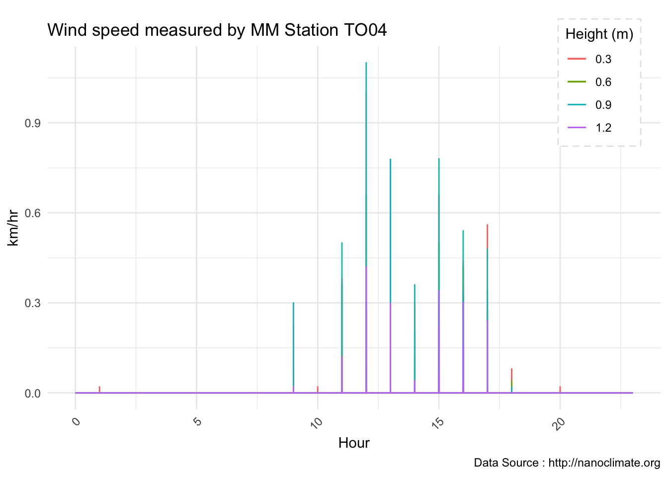
TO04
mclim_TO04_CN01_2018 %>% filter(month %in% c(9)) %>%
ggplot() +
geom_line( aes(hr,windspeed4,color = '0.3')) +
geom_line( aes(hr,windspeed3,color = '0.6')) +
geom_line( aes(hr,windspeed2,color = '0.9')) +
geom_line( aes(hr,windspeed1,color = '1.2')) +
theme_minimal() +
theme(legend.position = c(.9,.9),
legend.background = element_rect(color = "grey90",
size = .5, linetype = "dashed"),
axis.text.x=element_text(angle=45, hjust=1)) +
theme(strip.text.x = element_text(face="bold", size=12)) +
theme(strip.text.y = element_text(face="bold", size=12)) +
labs(title="Wind speed measured by MM Station TO04",x="Hour", y="km/hr", tag="", colour = "Height (m)",
caption="Data Source : http://nanoclimate.org")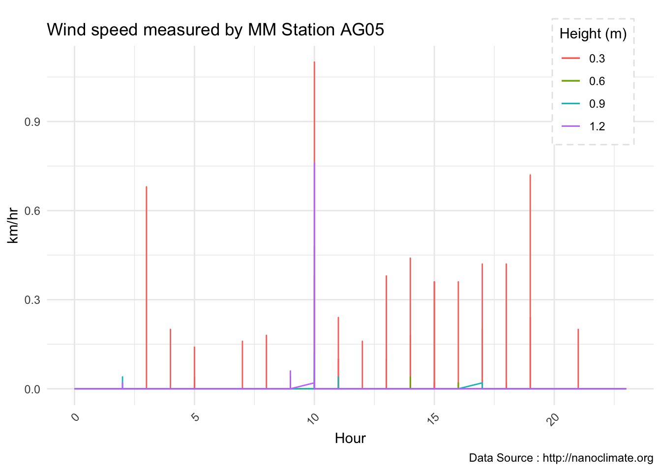
AG05
mclim_AG05_CN01_2018 %>% filter(month %in% c(9)) %>%
ggplot() +
geom_line( aes(hr,windspeed4,color = '0.3')) +
geom_line( aes(hr,windspeed3,color = '0.6')) +
geom_line( aes(hr,windspeed2,color = '0.9')) +
geom_line( aes(hr,windspeed1,color = '1.2')) +
theme_minimal() +
theme(legend.position = c(.9,.9),
legend.background = element_rect(color = "grey90",
size = .5, linetype = "dashed"),
axis.text.x=element_text(angle=45, hjust=1)) +
theme(strip.text.x = element_text(face="bold", size=12)) +
theme(strip.text.y = element_text(face="bold", size=12)) +
labs(title="Wind speed measured by MM Station AG05",x="Hour", y="km/hr", tag="", colour = "Height (m)",
caption="Data Source : http://nanoclimate.org")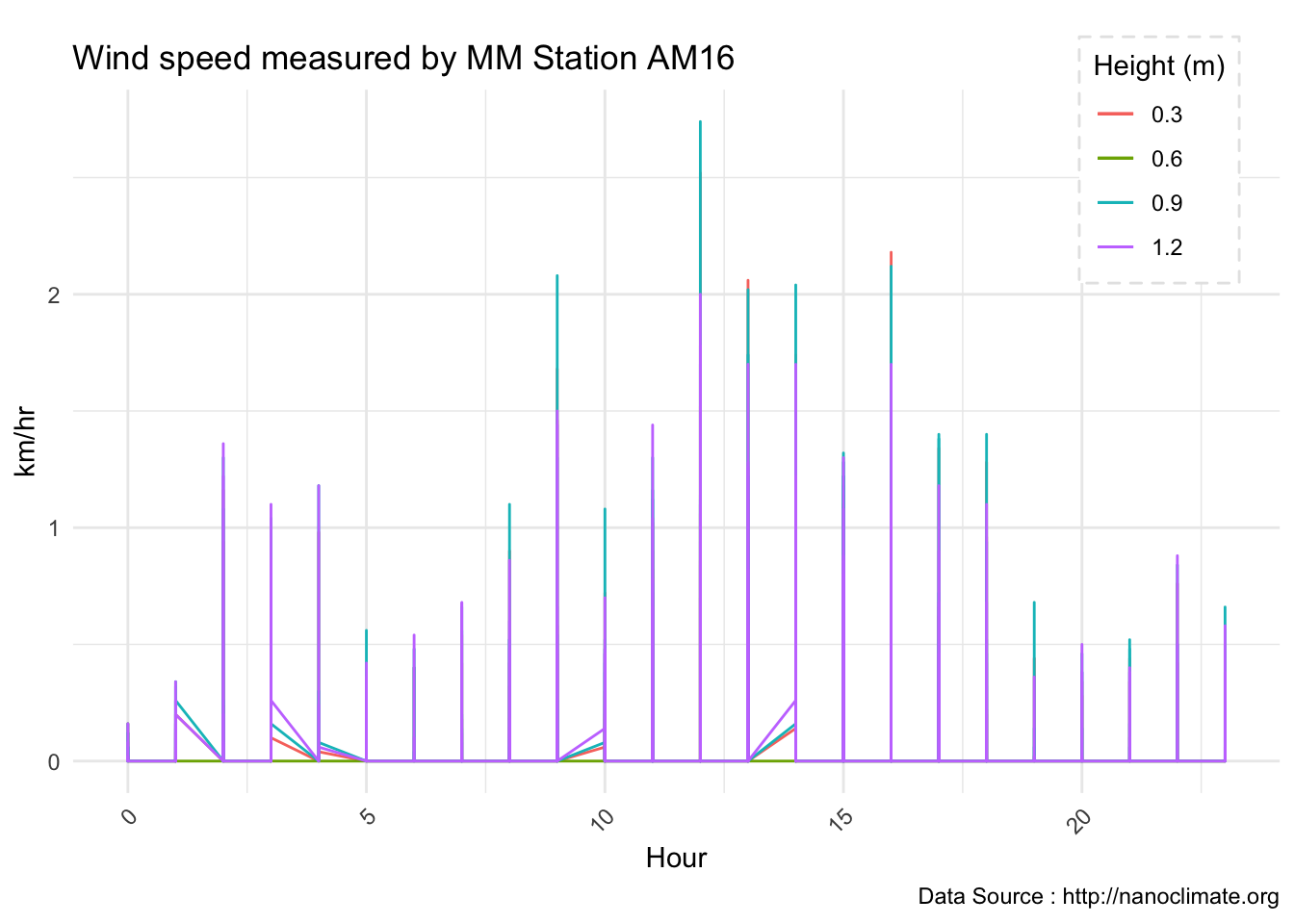
mclim_AM16_CN01_2018 %>% filter(month %in% c(9)) %>%
ggplot() +
geom_line( aes(hr,windspeed4,color = '0.3')) +
geom_line( aes(hr,windspeed3,color = '0.6')) +
geom_line( aes(hr,windspeed2,color = '0.9')) +
geom_line( aes(hr,windspeed1,color = '1.2')) +
theme_minimal() +
theme(legend.position = c(.9,.9),
legend.background = element_rect(color = "grey90",
size = .5, linetype = "dashed"),
axis.text.x=element_text(angle=45, hjust=1)) +
theme(strip.text.x = element_text(face="bold", size=12)) +
theme(strip.text.y = element_text(face="bold", size=12)) +
labs(title="Wind speed measured by MM Station AM16",x="Hour", y="km/hr", tag="", colour = "Height (m)",
caption="Data Source : http://nanoclimate.org")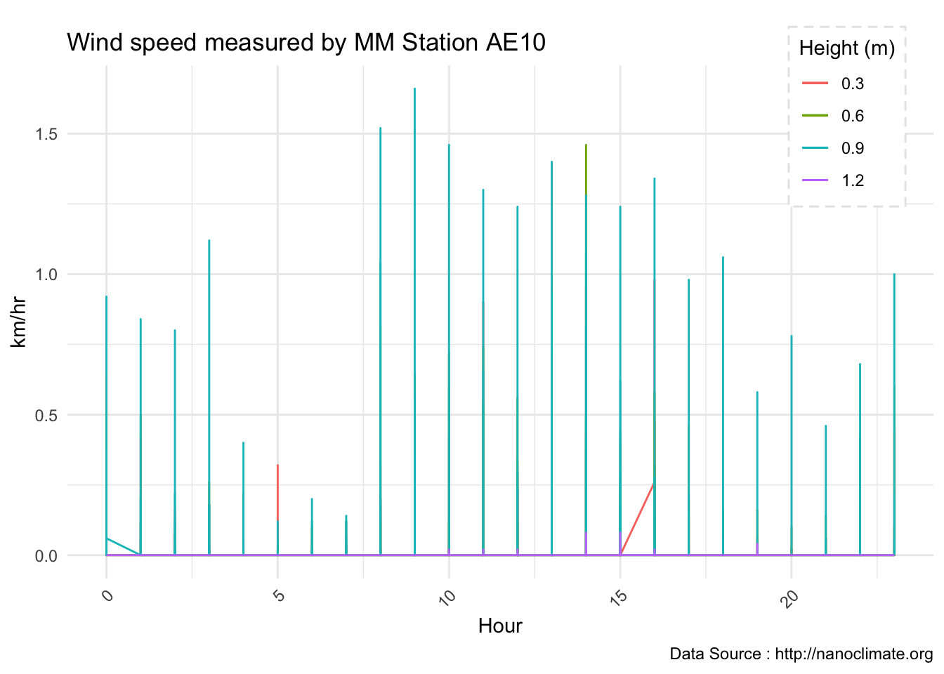
mclim_AE10_CN01_2018 %>% filter(month %in% c(9)) %>%
ggplot() +
geom_line( aes(hr,windspeed4,color = '0.3')) +
geom_line( aes(hr,windspeed3,color = '0.6')) +
geom_line( aes(hr,windspeed2,color = '0.9')) +
geom_line( aes(hr,windspeed1,color = '1.2')) +
theme_minimal() +
theme(legend.position = c(.9,.9),
legend.background = element_rect(color = "grey90",
size = .5, linetype = "dashed"),
axis.text.x=element_text(angle=45, hjust=1)) +
theme(strip.text.x = element_text(face="bold", size=12)) +
theme(strip.text.y = element_text(face="bold", size=12)) +
labs(title="Wind speed measured by MM Station AE10",x="Hour", y="km/hr", tag="", colour = "Height (m)",
caption="Data Source : http://nanoclimate.org")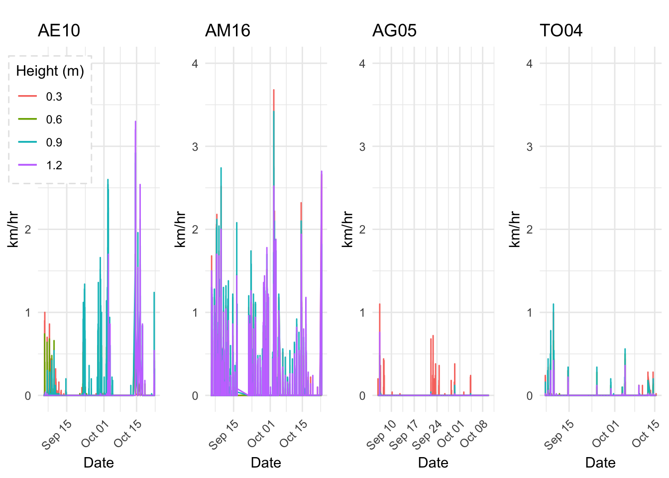
8.37 2-26-2019
Wind across 4 elevations at different heights
mw1 <- mclim_AE10_CN01_2018 %>% filter(month %in% c(9,10) & time > date('2018-09-05')) %>%
ggplot() +
geom_line( aes(time,windspeed4,color = '0.3')) +
geom_line( aes(time,windspeed3,color = '0.6')) +
geom_line( aes(time,windspeed2,color = '0.9')) +
geom_line( aes(time,windspeed1,color = '1.2')) +
theme_minimal() +
theme(legend.position = c(.1,.8),
legend.background = element_rect(color = "grey90",
size = .5, linetype = "dashed"),
axis.text.x=element_text(angle=45, hjust=1)) +
theme(strip.text.x = element_text(face="bold", size=12)) +
theme(strip.text.y = element_text(face="bold", size=12)) +
scale_y_continuous(limits = c(0, 4),breaks = c(0,1,2,3,4)) +
labs(title="AE10",x="Date", y="km/hr", tag="", colour = "Height (m)")
mw2 <- mclim_AM16_CN01_2018 %>% filter(month %in% c(9,10) & time > date('2018-09-05')) %>%
ggplot() +
geom_line( aes(time,windspeed4,color = '0.3')) +
geom_line( aes(time,windspeed3,color = '0.6')) +
geom_line( aes(time,windspeed2,color = '0.9')) +
geom_line( aes(time,windspeed1,color = '1.2')) +
theme_minimal() +
theme(legend.position="none",
legend.background = element_rect(color = "grey90",
size = .5, linetype = "dashed"),
axis.text.x=element_text(angle=45, hjust=1)) +
theme(strip.text.x = element_text(face="bold", size=12)) +
theme(strip.text.y = element_text(face="bold", size=12)) +
scale_y_continuous(limits = c(0, 4),breaks = c(0,1,2,3,4)) +
labs(title="AM16",x="Date", y="km/hr", tag="", colour = "Height (m)")
mw3 <- mclim_AG05_CN01_2018 %>% filter(month %in% c(9,10) & time > date('2018-09-05')) %>%
ggplot() +
geom_line( aes(time,windspeed4,color = '0.3')) +
geom_line( aes(time,windspeed3,color = '0.6')) +
geom_line( aes(time,windspeed2,color = '0.9')) +
geom_line( aes(time,windspeed1,color = '1.2')) +
theme_minimal() +
ylim(0,4) +
theme(legend.position="none",
legend.background = element_rect(color = "grey90",
size = .5, linetype = "dashed"),
axis.text.x=element_text(angle=45, hjust=1)) +
theme(strip.text.x = element_text(face="bold", size=12)) +
theme(strip.text.y = element_text(face="bold", size=12)) +
scale_y_continuous(limits = c(0, 4),breaks = c(0,1,2,3,4)) +
labs(title="AG05",x="Date", y="km/hr", tag="", colour = "Height (m)")## Scale for 'y' is already present. Adding another scale for 'y', which
## will replace the existing scale. mw4 <- mclim_TO04_CN01_2018 %>% filter(month %in% c(9,10) & time > date('2018-09-05')) %>%
ggplot() +
geom_line( aes(time,windspeed4,color = '0.3')) +
geom_line( aes(time,windspeed3,color = '0.6')) +
geom_line( aes(time,windspeed2,color = '0.9')) +
geom_line( aes(time,windspeed1,color = '1.2')) +
theme_minimal() +
theme(legend.position="none",
legend.background = element_rect(color = "grey90",
size = .5, linetype = "dashed"),
axis.text.x=element_text(angle=45, hjust=1)) +
theme(strip.text.x = element_text(face="bold", size=12)) +
theme(strip.text.y = element_text(face="bold", size=12)) +
scale_y_continuous(limits = c(0, 4),breaks = c(0,1,2,3,4)) +
labs(title="TO04",x="Date", y="km/hr", tag="", colour = "Height (m)")
library(cowplot)##
## Attaching package: 'cowplot'## The following object is masked from 'package:ggpubr':
##
## get_legend## The following object is masked from 'package:ggplot2':
##
## ggsave main_row_wind_ts <- plot_grid(mw1,mw2,mw3,mw4, align = "v", nrow = 1)
plot_grid(main_row_wind_ts ,nrow = 1)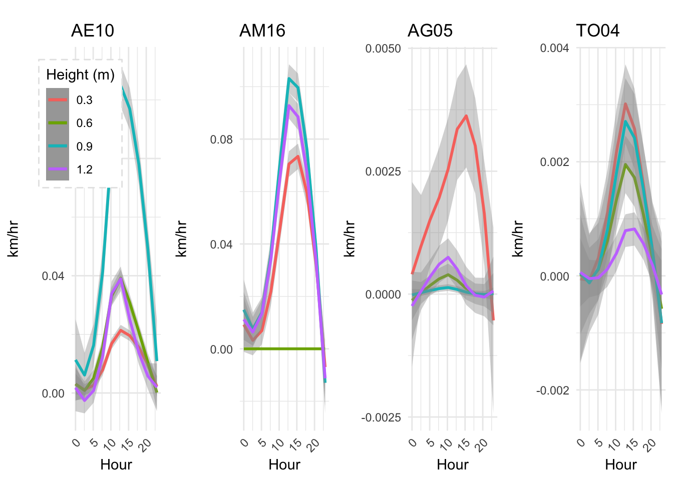
Wind at four heights , but hourly
mw1 <- mclim_AE10_CN01_2018 %>% filter(month %in% c(9,10) & time > date('2018-09-05')) %>%
ggplot() +
geom_smooth(method="loess" ,aes(hr,windspeed4,color = '0.3'),span = 0.8,n=10) +
geom_smooth(method="loess" ,aes(hr,windspeed3,color = '0.6'),span = 0.8,n=10) +
geom_smooth(method="loess" ,aes(hr,windspeed2,color = '0.9'),span = 0.8,n=10) +
geom_smooth(method="loess" ,aes(hr,windspeed1,color = '1.2'),span = 0.8,n=10) +
theme_minimal() +
theme(legend.position = c(.1,.8),
legend.background = element_rect(color = "grey90",
size = .5, linetype = "dashed"),
axis.text.x=element_text(angle=45, hjust=1)) +
theme(strip.text.x = element_text(face="bold", size=12)) +
theme(strip.text.y = element_text(face="bold", size=12)) +
labs(title="AE10",x="Hour", y="km/hr", tag="", colour = "Height (m)")
mw2 <- mclim_AM16_CN01_2018 %>% filter(month %in% c(9,10) & time > date('2018-09-05')) %>%
ggplot() +
geom_smooth(method="loess" ,aes(hr,windspeed4,color = '0.3'),span = 0.8,n=10) +
geom_smooth(method="loess" ,aes(hr,windspeed3,color = '0.6'),span = 0.8,n=10) +
geom_smooth(method="loess" ,aes(hr,windspeed2,color = '0.9'),span = 0.8,n=10) +
geom_smooth(method="loess" ,aes(hr,windspeed1,color = '1.2'),span = 0.8,n=10) +
theme_minimal() +
theme(legend.position="none",
legend.background = element_rect(color = "grey90",
size = .5, linetype = "dashed"),
axis.text.x=element_text(angle=45, hjust=1)) +
theme(strip.text.x = element_text(face="bold", size=12)) +
theme(strip.text.y = element_text(face="bold", size=12)) +
labs(title="AM16",x="Hour", y="km/hr", tag="", colour = "Height (m)")
mw3 <- mclim_AG05_CN01_2018 %>% filter(month %in% c(9,10) & time > date('2018-09-05')) %>%
ggplot() +
geom_smooth(method="loess" ,aes(hr,windspeed4,color = '0.3'),span = 0.8,n=10) +
geom_smooth(method="loess" ,aes(hr,windspeed3,color = '0.6'),span = 0.8,n=10) +
geom_smooth(method="loess" ,aes(hr,windspeed2,color = '0.9'),span = 0.8,n=10) +
geom_smooth(method="loess" ,aes(hr,windspeed1,color = '1.2'),span = 0.8,n=10) +
theme_minimal() +
theme(legend.position="none",
legend.background = element_rect(color = "grey90",
size = .5, linetype = "dashed"),
axis.text.x=element_text(angle=45, hjust=1)) +
theme(strip.text.x = element_text(face="bold", size=12)) +
theme(strip.text.y = element_text(face="bold", size=12)) +
labs(title="AG05",x="Hour", y="km/hr", tag="", colour = "Height (m)")
mw4 <- mclim_TO04_CN01_2018 %>% filter(month %in% c(9,10) & time > date('2018-09-05')) %>%
ggplot() +
geom_smooth(method="loess" ,aes(hr,windspeed4,color = '0.3'),span = 0.8,n=10) +
geom_smooth(method="loess" ,aes(hr,windspeed3,color = '0.6'),span = 0.8,n=10) +
geom_smooth(method="loess" ,aes(hr,windspeed2,color = '0.9'),span = 0.8,n=10) +
geom_smooth(method="loess" ,aes(hr,windspeed1,color = '1.2'),span = 0.8,n=10) +
theme_minimal() +
theme(legend.position="none",
legend.background = element_rect(color = "grey90",
size = .5, linetype = "dashed"),
axis.text.x=element_text(angle=45, hjust=1)) +
theme(strip.text.x = element_text(face="bold", size=12)) +
theme(strip.text.y = element_text(face="bold", size=12)) +
labs(title="TO04",x="Hour", y="km/hr", tag="", colour = "Height (m)")
library(cowplot)
main_row_wind_hr <- plot_grid(mw1,mw2,mw3,mw4, align = "v", nrow = 1)
plot_grid(main_row_wind_hr ,nrow = 1)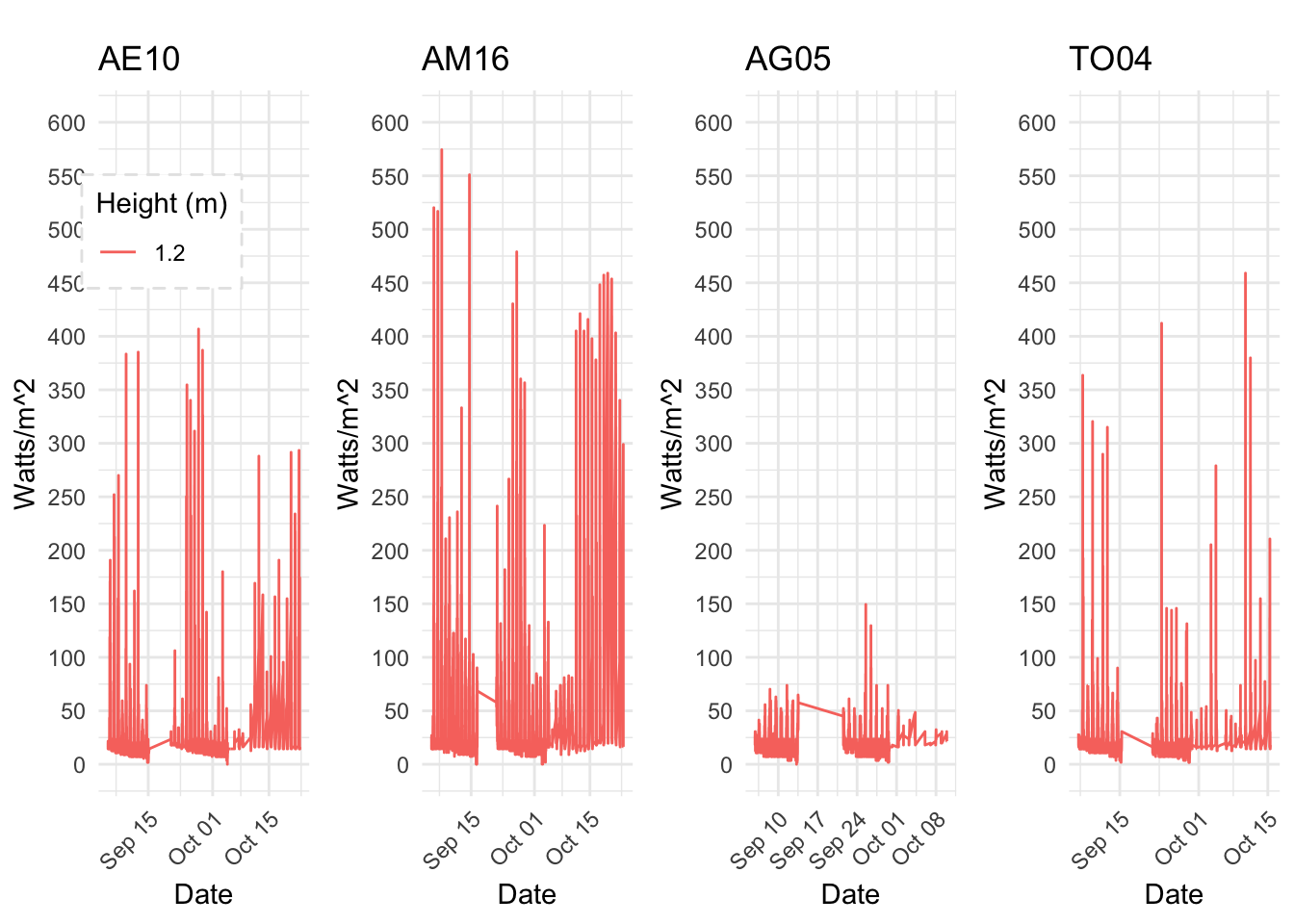
Solar radiation at 4 different heights
Wind across 4 elevations at different elevations , one height
mw1 <- mclim_AE10_CN01_2018 %>% filter(month %in% c(9,10) & time > date('2018-09-05')) %>%
mutate(solrf = ((solar-39) * 1.8) + ((25 -temp1) * .0012)) %>%
ggplot() +
geom_line( aes(time,solrf,color = '1.2')) +
theme_minimal() +
theme(legend.position = c(.3,.8),
legend.background = element_rect(color = "grey90",
size = .5, linetype = "dashed"),
axis.text.x=element_text(angle=45, hjust=1)) +
theme(strip.text.x = element_text(face="bold", size=12)) +
theme(strip.text.y = element_text(face="bold", size=12)) +
scale_y_continuous(limits = c(0, 600),breaks = c(0,50,100,150,200,250,300,350,400,450,500,550,600)) +
labs(title="AE10",x="Date", y="Watts/m^2", tag="", colour = "Height (m)")
mw2 <- mclim_AM16_CN01_2018 %>% filter(month %in% c(9,10) & time > date('2018-09-05')) %>%
mutate(solrf = ((solar-39) * 1.8) + ((25 -temp1) * .0012)) %>%
ggplot() +
geom_line( aes(time,solrf,color = '1.2')) +
theme_minimal() +
theme(legend.position="none",
legend.background = element_rect(color = "grey90",
size = .5, linetype = "dashed"),
axis.text.x=element_text(angle=45, hjust=1)) +
theme(strip.text.x = element_text(face="bold", size=12)) +
theme(strip.text.y = element_text(face="bold", size=12)) +
scale_y_continuous(limits = c(0, 600),breaks = c(0,50,100,150,200,250,300,350,400,450,500,550,600)) +
labs(title="AM16",x="Date", y="Watts/m^2", tag="", colour = "Height (m)")
mw3 <- mclim_AG05_CN01_2018 %>% filter(month %in% c(9,10) & time > date('2018-09-05')) %>%
mutate(solrf = ((solar-39) * 1.8) + ((25 -temp1) * .0012)) %>%
ggplot() +
geom_line( aes(time,solrf,color = '1.2')) +
theme_minimal() +
ylim(0,4) +
theme(legend.position="none",
legend.background = element_rect(color = "grey90",
size = .5, linetype = "dashed"),
axis.text.x=element_text(angle=45, hjust=1)) +
theme(strip.text.x = element_text(face="bold", size=12)) +
theme(strip.text.y = element_text(face="bold", size=12)) +
scale_y_continuous(limits = c(0, 600),breaks = c(0,50,100,150,200,250,300,350,400,450,500,550,600)) +
labs(title="AG05",x="Date", y="Watts/m^2", tag="", colour = "Height (m)")## Scale for 'y' is already present. Adding another scale for 'y', which
## will replace the existing scale. mw4 <- mclim_TO04_CN01_2018 %>% filter(month %in% c(9,10) & time > date('2018-09-05')) %>%
mutate(solrf = ((solar-39) * 1.8) + ((25 -temp1) * .0012)) %>%
ggplot() +
geom_line( aes(time,solrf,color = '1.2')) +
theme_minimal() +
theme(legend.position="none",
legend.background = element_rect(color = "grey90",
size = .5, linetype = "dashed"),
axis.text.x=element_text(angle=45, hjust=1)) +
theme(strip.text.x = element_text(face="bold", size=12)) +
theme(strip.text.y = element_text(face="bold", size=12)) +
scale_y_continuous(limits = c(0, 600),breaks = c(0,50,100,150,200,250,300,350,400,450,500,550,600)) +
labs(title="TO04",x="Date", y="Watts/m^2", tag="", colour = "Height (m)")
library(cowplot)
main_row_ts <- plot_grid(mw1,mw2,mw3,mw4, align = "v", nrow = 1)
plot_grid(main_row_ts ,nrow = 1)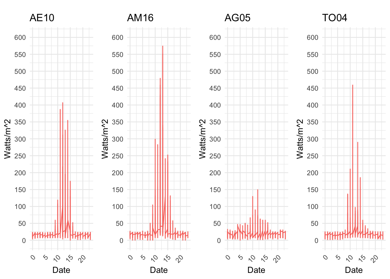
8.38 2-27-2019
Need to see spread of solar radation by hour, and do we see prolonged period of illumination?
I believe the reduced solar radiation penetration reflects on the distribution and nature of understory vegetation. Most of the understories are varied, and the ones are prominent in the confiers are very dry, and the ones which are close to water exhibit ferns, and similar kind of bog loving vegetation (personal observation). Its also possible that they are adapted to reduced avaliability of radiation.
Hourly radiation load
mw1 <- mclim_AE10_CN01_2018 %>% filter(month %in% c(9,10) & time > date('2018-09-05')) %>%
mutate(solrf = ((solar-39) * 1.8) + ((25 -temp1) * .0012)) %>%
ggplot() +
geom_line( aes(hr,solrf,color = '1.2')) +
theme_minimal() +
theme(legend.position = "none",
legend.background = element_rect(color = "grey90",
size = .5, linetype = "dashed"),
axis.text.x=element_text(angle=45, hjust=1)) +
theme(strip.text.x = element_text(face="bold", size=12)) +
theme(strip.text.y = element_text(face="bold", size=12)) +
scale_y_continuous(limits = c(0, 600),breaks = c(0,50,100,150,200,250,300,350,400,450,500,550,600)) +
labs(title="AE10",x="Date", y="Watts/m^2", tag="", colour = "Height (m)")
mw2 <- mclim_AM16_CN01_2018 %>% filter(month %in% c(9,10) & time > date('2018-09-05')) %>%
mutate(solrf = ((solar-39) * 1.8) + ((25 -temp1) * .0012)) %>%
ggplot() +
geom_line( aes(hr,solrf,color = '1.2')) +
theme_minimal() +
theme(legend.position="none",
legend.background = element_rect(color = "grey90",
size = .5, linetype = "dashed"),
axis.text.x=element_text(angle=45, hjust=1)) +
theme(strip.text.x = element_text(face="bold", size=12)) +
theme(strip.text.y = element_text(face="bold", size=12)) +
scale_y_continuous(limits = c(0, 600),breaks = c(0,50,100,150,200,250,300,350,400,450,500,550,600)) +
labs(title="AM16",x="Date", y="Watts/m^2", tag="", colour = "Height (m)")
mw3 <- mclim_AG05_CN01_2018 %>% filter(month %in% c(9,10) & time > date('2018-09-05')) %>%
mutate(solrf = ((solar-39) * 1.8) + ((25 -temp1) * .0012)) %>%
ggplot() +
geom_line( aes(hr,solrf,color = '1.2')) +
theme_minimal() +
ylim(0,4) +
theme(legend.position="none",
legend.background = element_rect(color = "grey90",
size = .5, linetype = "dashed"),
axis.text.x=element_text(angle=45, hjust=1)) +
theme(strip.text.x = element_text(face="bold", size=12)) +
theme(strip.text.y = element_text(face="bold", size=12)) +
scale_y_continuous(limits = c(0, 600),breaks = c(0,50,100,150,200,250,300,350,400,450,500,550,600)) +
labs(title="AG05",x="Date", y="Watts/m^2", tag="", colour = "Height (m)")## Scale for 'y' is already present. Adding another scale for 'y', which
## will replace the existing scale. mw4 <- mclim_TO04_CN01_2018 %>% filter(month %in% c(9,10) & time > date('2018-09-05')) %>%
mutate(solrf = ((solar-39) * 1.8) + ((25 -temp1) * .0012)) %>%
ggplot() +
geom_line( aes(hr,solrf,color = '1.2')) +
theme_minimal() +
theme(legend.position="none",
legend.background = element_rect(color = "grey90",
size = .5, linetype = "dashed"),
axis.text.x=element_text(angle=45, hjust=1)) +
theme(strip.text.x = element_text(face="bold", size=12)) +
theme(strip.text.y = element_text(face="bold", size=12)) +
scale_y_continuous(limits = c(0, 600),breaks = c(0,50,100,150,200,250,300,350,400,450,500,550,600)) +
labs(title="TO04",x="Date", y="Watts/m^2", tag="", colour = "Height (m)")
library(cowplot)
main_row <- plot_grid(mw1,mw2,mw3,mw4, align = "v", nrow = 1)
plot_grid(main_row ,nrow = 1)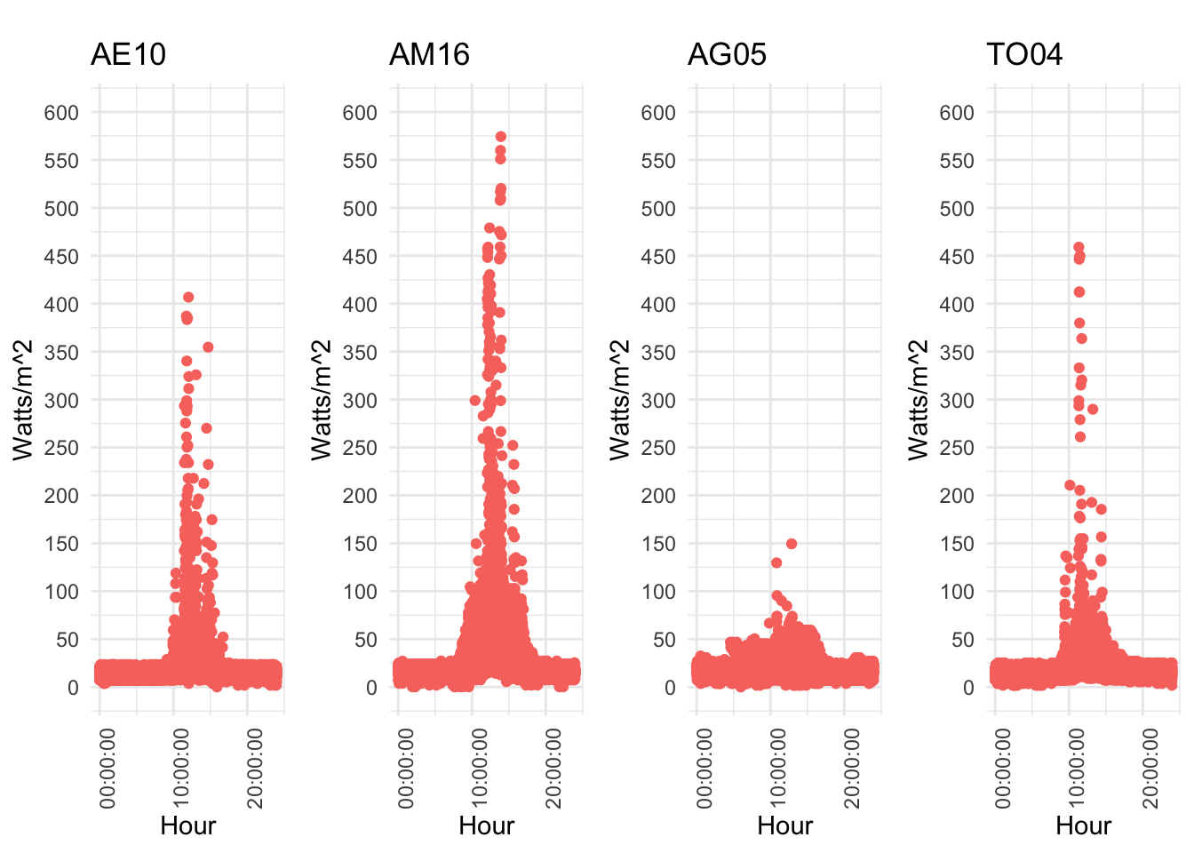
Find the duration as literature says that topical forests receive 5-10 mins, and temperates should be an hour. I believe, this should be qualified with the opening.
mw1 <- mclim_AE10_CN01_2018 %>% filter(month %in% c(9,10) & time > date('2018-09-05')) %>%
mutate(solrf = ((solar-39) * 1.8) + ((25 -temp1) * .0012)) %>%
mutate(hm = as.POSIXct( paste(hr,minute,sep = ':') , format = "%H:%M")) %>%
mutate(hms = hms::as.hms(hm)) %>%
ggplot() +
#geom_line( aes(hr,solrf,color = '1.2')) +
geom_point(aes(hms,solrf,color = '1.2')) +
theme_minimal() +
theme(legend.position = "none",
legend.background = element_rect(color = "grey90",
size = .5, linetype = "dashed"),
axis.text.x=element_text(angle=90, hjust=1)) +
scale_y_continuous(limits = c(0, 600),breaks = c(0,50,100,150,200,250,300,350,400,450,500,550,600)) +
scale_x_time(labels=date_format("%H:%M")) +
labs(title="AE10",x="Hour", y="Watts/m^2", tag="", colour = "Height (m)")
mw2 <- mclim_AM16_CN01_2018 %>% filter(month %in% c(9,10) & time > date('2018-09-05')) %>%
mutate(solrf = ((solar-39) * 1.8) + ((25 -temp1) * .0012)) %>%
mutate(hm = as.POSIXct( paste(hr,minute,sep = ':') , format = "%H:%M")) %>%
mutate(hms = hms::as.hms(hm)) %>%
ggplot() +
#geom_line( aes(hr,solrf,color = '1.2')) +
geom_point(aes(hms,solrf,color = '1.2')) +
theme_minimal() +
theme(legend.position = "none",
legend.background = element_rect(color = "grey90",
size = .5, linetype = "dashed"),
axis.text.x=element_text(angle=90, hjust=1)) +
scale_y_continuous(limits = c(0, 600),breaks = c(0,50,100,150,200,250,300,350,400,450,500,550,600)) +
scale_x_time(labels=date_format("%H:%M")) +
labs(title="AM16",x="Hour", y="Watts/m^2", tag="", colour = "Height (m)")
mw3 <- mclim_AG05_CN01_2018 %>% filter(month %in% c(9,10) & time > date('2018-09-05')) %>%
mutate(solrf = ((solar-39) * 1.8) + ((25 -temp1) * .0012)) %>%
mutate(hm = as.POSIXct( paste(hr,minute,sep = ':') , format = "%H:%M")) %>%
mutate(hms = hms::as.hms(hm)) %>%
ggplot() +
#geom_line( aes(hr,solrf,color = '1.2')) +
geom_point(aes(hms,solrf,color = '1.2')) +
theme_minimal() +
theme(legend.position = "none",
legend.background = element_rect(color = "grey90",
size = .5, linetype = "dashed"),
axis.text.x=element_text(angle=90, hjust=1)) +
scale_y_continuous(limits = c(0, 600),breaks = c(0,50,100,150,200,250,300,350,400,450,500,550,600)) +
scale_x_time(labels=date_format("%H:%M")) +
labs(title="AG05",x="Hour", y="Watts/m^2", tag="", colour = "Height (m)")
mw4 <- mclim_TO04_CN01_2018 %>% filter(month %in% c(9,10) & time > date('2018-09-05')) %>%
mutate(solrf = ((solar-39) * 1.8) + ((25 -temp1) * .0012)) %>%
mutate(hm = as.POSIXct( paste(hr,minute,sep = ':') , format = "%H:%M")) %>%
mutate(hms = hms::as.hms(hm)) %>%
ggplot() +
#geom_line( aes(hr,solrf,color = '1.2')) +
geom_point(aes(hms,solrf,color = '1.2')) +
theme_minimal() +
theme(legend.position = "none",
legend.background = element_rect(color = "grey90",
size = .5, linetype = "dashed"),
axis.text.x=element_text(angle=90, hjust=1)) +
scale_y_continuous(limits = c(0, 600),breaks = c(0,50,100,150,200,250,300,350,400,450,500,550,600)) +
scale_x_time(labels=date_format("%H:%M")) +
labs(title="TO04",x="Hour", y="Watts/m^2", tag="", colour = "Height (m)")
library(cowplot)
main_row_hr <- plot_grid(mw1,mw2,mw3,mw4, align = "v", nrow = 1)
plot_grid(main_row_hr ,nrow = 1)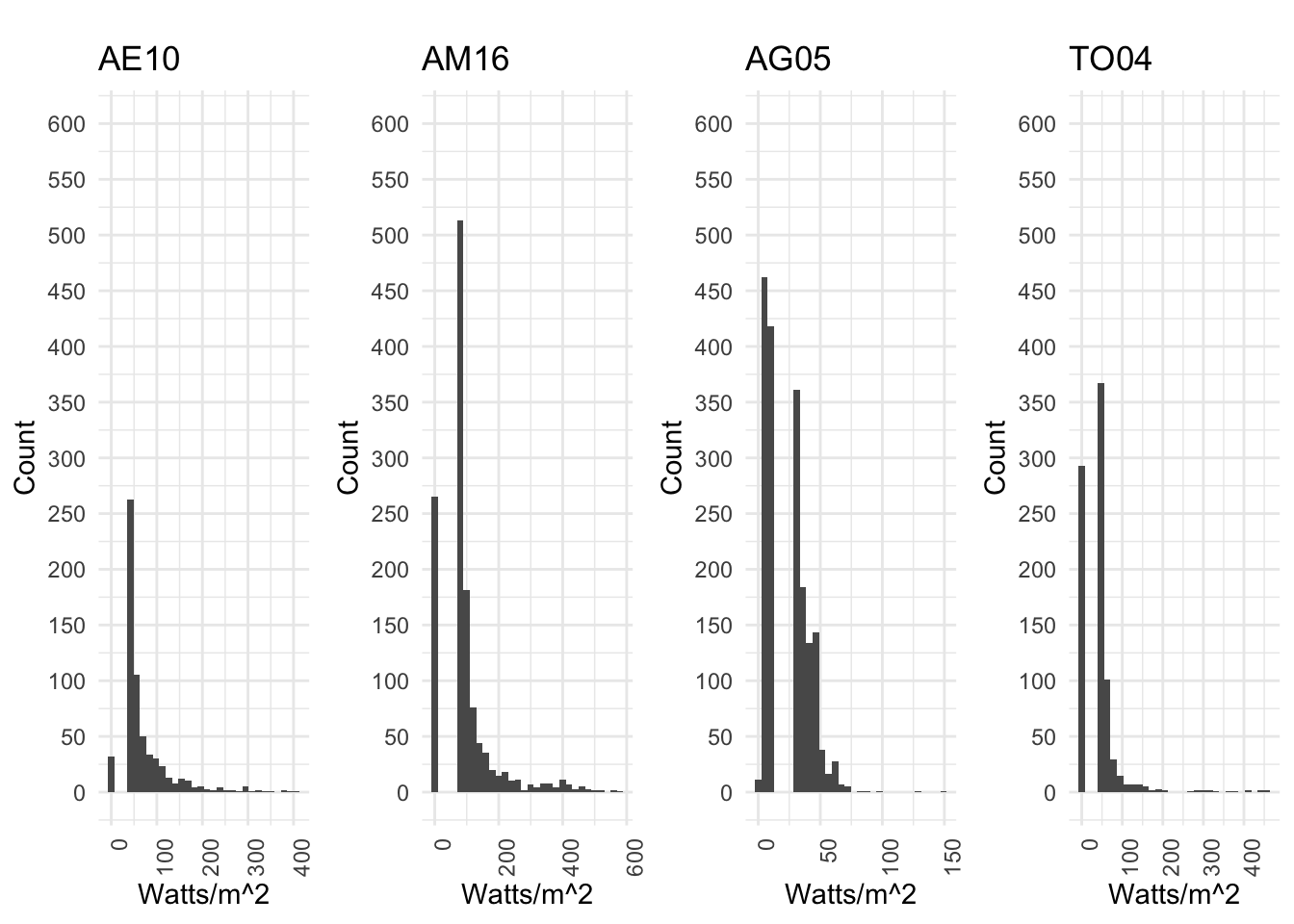
Histogram
mw1 <- mclim_AE10_CN01_2018 %>% filter(month %in% c(9,10) & time > date('2018-09-05')) %>%
mutate(solrf = ((solar-39) * 1.8) + ((25 -temp1) * .0012)) %>%
mutate(hm = as.POSIXct( paste(hr,minute,sep = ':') , format = "%H:%M")) %>%
mutate(hms = hms::as.hms(hm)) %>%
ggplot() +
#geom_line( aes(hr,solrf,color = '1.2')) +
geom_histogram(aes(solrf)) +
theme_minimal() +
theme(legend.position = "none",
legend.background = element_rect(color = "grey90",
size = .5, linetype = "dashed"),
axis.text.x=element_text(angle=90, hjust=1)) +
scale_y_continuous(limits = c(0, 600),breaks = c(0,50,100,150,200,250,300,350,400,450,500,550,600)) +
labs(title="AE10",x="Watts/m^2", y="Count", tag="", colour = "")
mw2 <- mclim_AM16_CN01_2018 %>% filter(month %in% c(9,10) & time > date('2018-09-05')) %>%
mutate(solrf = ((solar-39) * 1.8) + ((25 -temp1) * .0012)) %>%
mutate(hm = as.POSIXct( paste(hr,minute,sep = ':') , format = "%H:%M")) %>%
mutate(hms = hms::as.hms(hm)) %>%
ggplot() +
#geom_line( aes(hr,solrf,color = '1.2')) +
geom_histogram(aes(solrf)) +
theme_minimal() +
theme(legend.position = "none",
legend.background = element_rect(color = "grey90",
size = .5, linetype = "dashed"),
axis.text.x=element_text(angle=90, hjust=1)) +
scale_y_continuous(limits = c(0, 600),breaks = c(0,50,100,150,200,250,300,350,400,450,500,550,600)) +
labs(title="AM16",x="Watts/m^2", y="Count", tag="", colour = "")
mw3 <- mclim_AG05_CN01_2018 %>% filter(month %in% c(9,10) & time > date('2018-09-05')) %>%
mutate(solrf = ((solar-39) * 1.8) + ((25 -temp1) * .0012)) %>%
mutate(hm = as.POSIXct( paste(hr,minute,sep = ':') , format = "%H:%M")) %>%
mutate(hms = hms::as.hms(hm)) %>%
ggplot() +
#geom_line( aes(hr,solrf,color = '1.2')) +
geom_histogram(aes(solrf)) +
theme_minimal() +
theme(legend.position = "none",
legend.background = element_rect(color = "grey90",
size = .5, linetype = "dashed"),
axis.text.x=element_text(angle=90, hjust=1)) +
scale_y_continuous(limits = c(0, 600),breaks = c(0,50,100,150,200,250,300,350,400,450,500,550,600)) +
labs(title="AG05", x="Watts/m^2", y="Count", tag="", colour = "")
mw4 <- mclim_TO04_CN01_2018 %>% filter(month %in% c(9,10) & time > date('2018-09-05')) %>%
mutate(solrf = ((solar-39) * 1.8) + ((25 -temp1) * .0012)) %>%
mutate(hm = as.POSIXct( paste(hr,minute,sep = ':') , format = "%H:%M")) %>%
mutate(hms = hms::as.hms(hm)) %>%
ggplot() +
#geom_line( aes(hr,solrf,color = '1.2')) +
geom_histogram(aes(solrf)) +
theme_minimal() +
theme(legend.position = "none",
legend.background = element_rect(color = "grey90",
size = .5, linetype = "dashed"),
axis.text.x=element_text(angle=90, hjust=1)) +
scale_y_continuous(limits = c(0, 600),breaks = c(0,50,100,150,200,250,300,350,400,450,500,550,600)) +
labs(title="TO04",x="Watts/m^2", y="Count", tag="", colour = "")
library(cowplot)
main_row_hst <- plot_grid(mw1,mw2,mw3,mw4, align = "v", nrow = 1)## `stat_bin()` using `bins = 30`. Pick better value with `binwidth`.
## `stat_bin()` using `bins = 30`. Pick better value with `binwidth`.
## `stat_bin()` using `bins = 30`. Pick better value with `binwidth`.
## `stat_bin()` using `bins = 30`. Pick better value with `binwidth`. plot_grid(main_row_hst ,nrow = 1)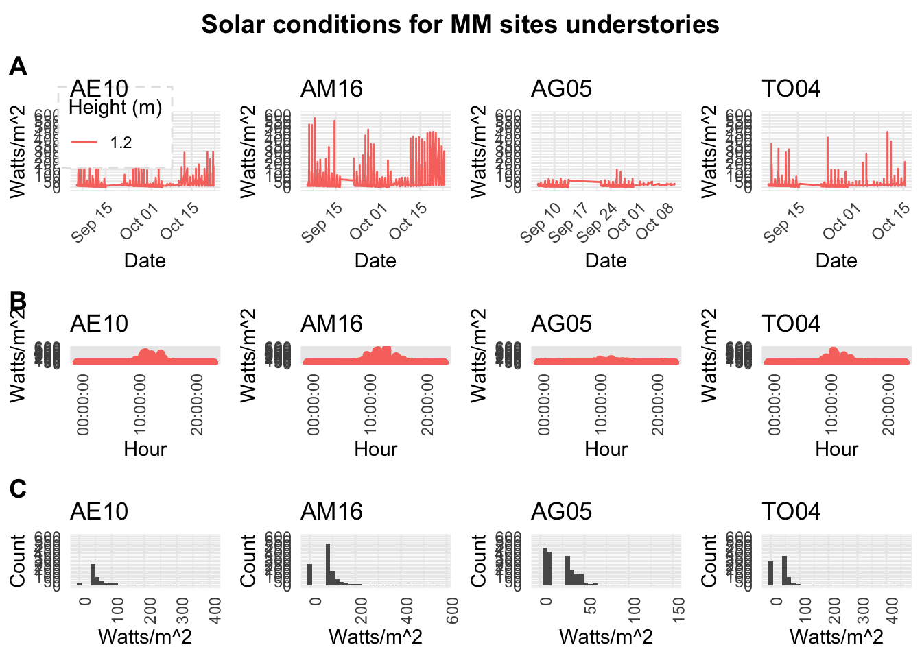
8.39 3-1-2019
Combined Panel Solar
title <- ggdraw() + draw_label("Solar conditions for MM sites understories", fontface='bold')
plot_grid(title, main_row_ts,main_row_hr, main_row_hst, nrow = 4, labels = c("", "A","B", "C"),
rel_heights = c(0.2, 1,.8, .8))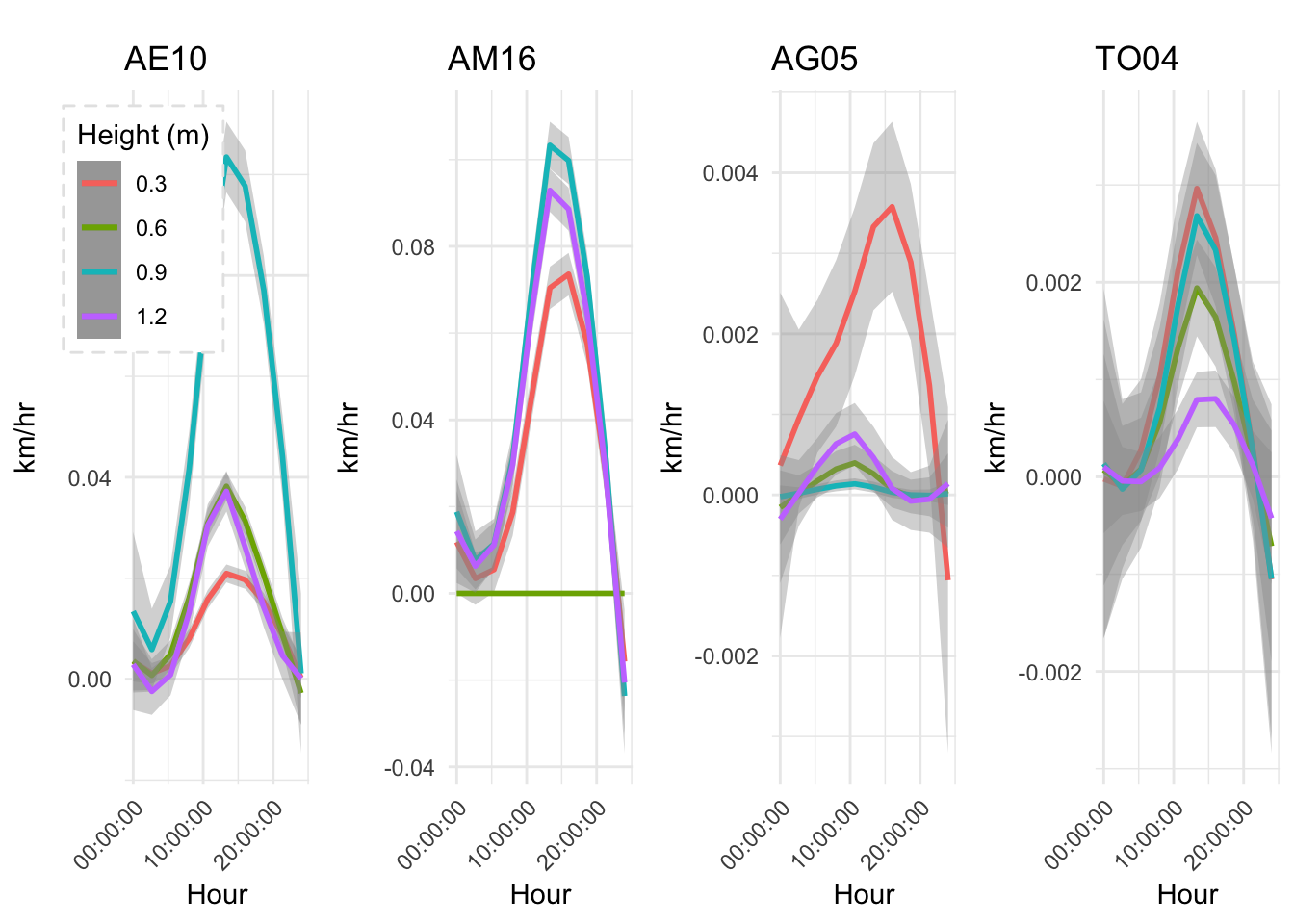
Wind
mw1 <- mclim_AE10_CN01_2018 %>% filter(month %in% c(9,10) & time > date('2018-09-05')) %>%
mutate(hm = as.POSIXct( paste(hr,minute,sep = ':') , format = "%H:%M")) %>%
mutate(hms = hms::as.hms(hm)) %>%
ggplot() +
geom_smooth(method="loess" ,aes(hms,windspeed4,color = '0.3'),span = 0.8,n=10) +
geom_smooth(method="loess" ,aes(hms,windspeed3,color = '0.6'),span = 0.8,n=10) +
geom_smooth(method="loess" ,aes(hms,windspeed2,color = '0.9'),span = 0.8,n=10) +
geom_smooth(method="loess" ,aes(hms,windspeed1,color = '1.2'),span = 0.8,n=10) +
theme_minimal() +
theme(legend.position = c(.1,.8),
legend.background = element_rect(color = "grey90",
size = .5, linetype = "dashed"),
axis.text.x=element_text(angle=45, hjust=1)) +
theme(strip.text.x = element_text(face="bold", size=12)) +
theme(strip.text.y = element_text(face="bold", size=12)) +
labs(title="AE10",x="Hour", y="km/hr", tag="", colour = "Height (m)")
mw2 <- mclim_AM16_CN01_2018 %>% filter(month %in% c(9,10) & time > date('2018-09-05')) %>%
mutate(hm = as.POSIXct( paste(hr,minute,sep = ':') , format = "%H:%M")) %>%
mutate(hms = hms::as.hms(hm)) %>%
ggplot() +
geom_smooth(method="loess" ,aes(hms,windspeed4,color = '0.3'),span = 0.8,n=10) +
geom_smooth(method="loess" ,aes(hms,windspeed3,color = '0.6'),span = 0.8,n=10) +
geom_smooth(method="loess" ,aes(hms,windspeed2,color = '0.9'),span = 0.8,n=10) +
geom_smooth(method="loess" ,aes(hms,windspeed1,color = '1.2'),span = 0.8,n=10) +
theme_minimal() +
theme(legend.position="none",
legend.background = element_rect(color = "grey90",
size = .5, linetype = "dashed"),
axis.text.x=element_text(angle=45, hjust=1)) +
theme(strip.text.x = element_text(face="bold", size=12)) +
theme(strip.text.y = element_text(face="bold", size=12)) +
labs(title="AM16",x="Hour", y="km/hr", tag="", colour = "Height (m)")
mw3 <- mclim_AG05_CN01_2018 %>% filter(month %in% c(9,10) & time > date('2018-09-05')) %>%
mutate(hm = as.POSIXct( paste(hr,minute,sep = ':') , format = "%H:%M")) %>%
mutate(hms = hms::as.hms(hm)) %>%
ggplot() +
geom_smooth(method="loess" ,aes(hms,windspeed4,color = '0.3'),span = 0.8,n=10) +
geom_smooth(method="loess" ,aes(hms,windspeed3,color = '0.6'),span = 0.8,n=10) +
geom_smooth(method="loess" ,aes(hms,windspeed2,color = '0.9'),span = 0.8,n=10) +
geom_smooth(method="loess" ,aes(hms,windspeed1,color = '1.2'),span = 0.8,n=10) +
theme_minimal() +
theme(legend.position="none",
legend.background = element_rect(color = "grey90",
size = .5, linetype = "dashed"),
axis.text.x=element_text(angle=45, hjust=1)) +
theme(strip.text.x = element_text(face="bold", size=12)) +
theme(strip.text.y = element_text(face="bold", size=12)) +
labs(title="AG05",x="Hour", y="km/hr", tag="", colour = "Height (m)")
mw4 <- mclim_TO04_CN01_2018 %>% filter(month %in% c(9,10) & time > date('2018-09-05')) %>%
mutate(hm = as.POSIXct( paste(hr,minute,sep = ':') , format = "%H:%M")) %>%
mutate(hms = hms::as.hms(hm)) %>%
ggplot() +
geom_smooth(method="loess" ,aes(hms,windspeed4,color = '0.3'),span = 0.8,n=10) +
geom_smooth(method="loess" ,aes(hms,windspeed3,color = '0.6'),span = 0.8,n=10) +
geom_smooth(method="loess" ,aes(hms,windspeed2,color = '0.9'),span = 0.8,n=10) +
geom_smooth(method="loess" ,aes(hms,windspeed1,color = '1.2'),span = 0.8,n=10) +
theme_minimal() +
theme(legend.position="none",
legend.background = element_rect(color = "grey90",
size = .5, linetype = "dashed"),
axis.text.x=element_text(angle=45, hjust=1)) +
theme(strip.text.x = element_text(face="bold", size=12)) +
theme(strip.text.y = element_text(face="bold", size=12)) +
labs(title="TO04",x="Hour", y="km/hr", tag="", colour = "Height (m)")
library(cowplot)
main_row_wind_hms <- plot_grid(mw1,mw2,mw3,mw4, align = "v", nrow = 1)
plot_grid(main_row_wind_hms ,nrow = 1)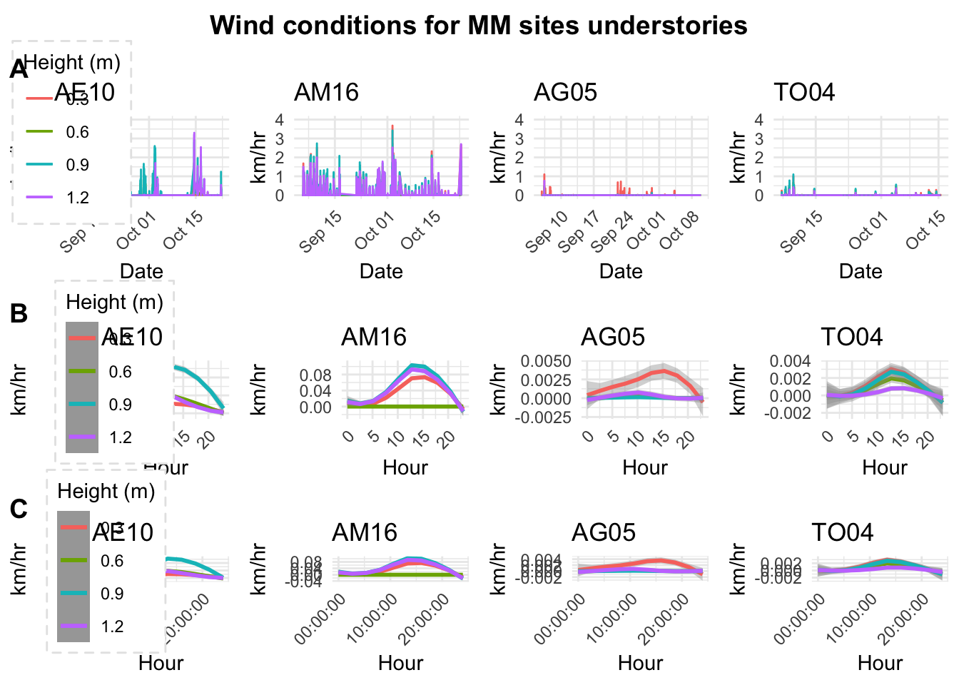
title <- ggdraw() + draw_label("Wind conditions for MM sites understories", fontface='bold')
plot_grid(title, main_row_wind_ts,main_row_wind_hr, main_row_wind_hms, nrow = 4, labels = c("", "A","B", "C"),
rel_heights = c(0.2, 1,.8, .8))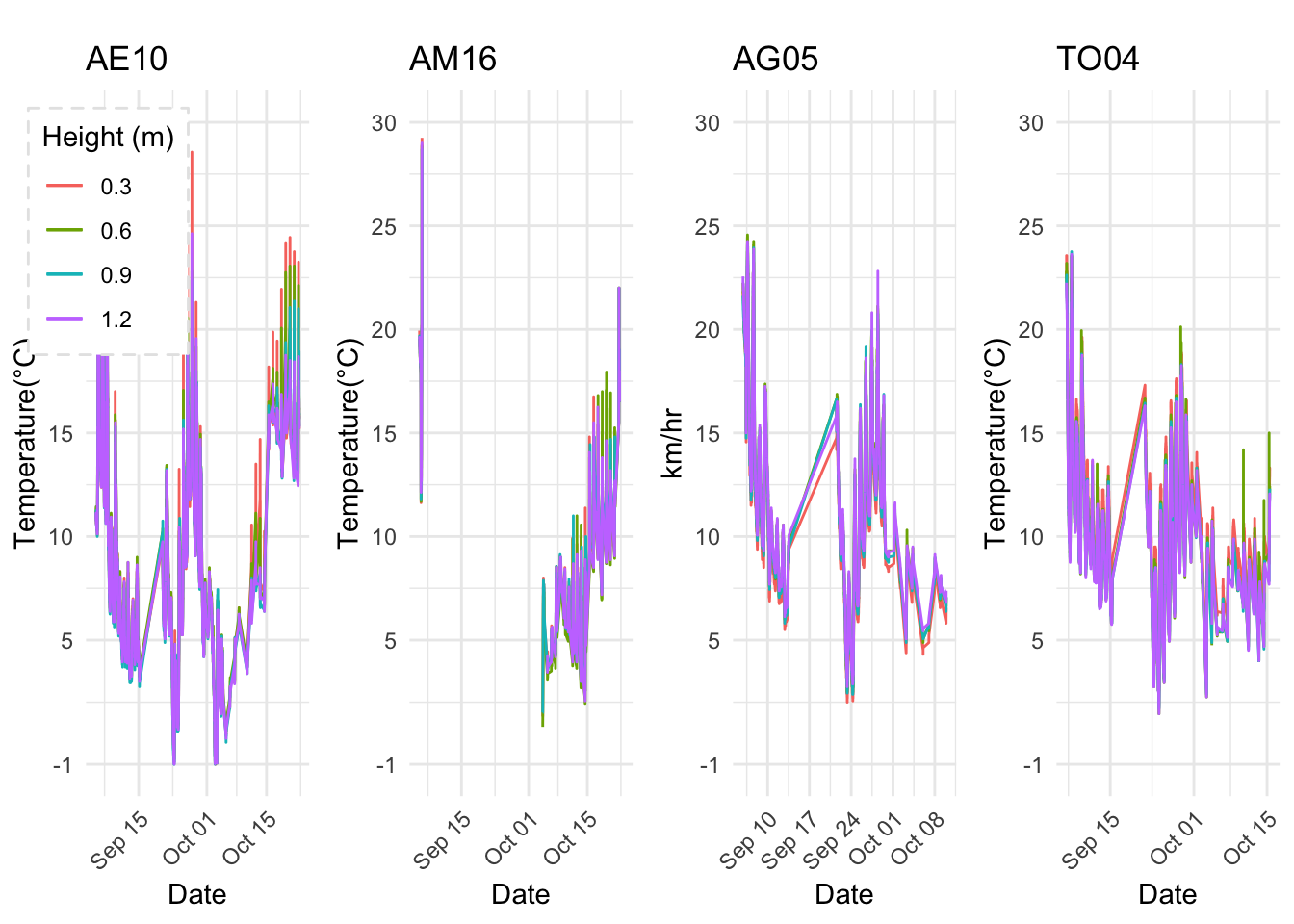
8.40 3-3-2019
Temperature stability assessment, different heights i.e. vertically.
First raw plots
mw1 <- mclim_AE10_CN01_2018 %>% filter(month %in% c(9,10) & time > date('2018-09-05')) %>%
ggplot() +
geom_line( aes(time,temp4,color = '0.3')) +
geom_line( aes(time,temp3,color = '0.6')) +
geom_line( aes(time,temp2,color = '0.9')) +
geom_line( aes(time,temp1,color = '1.2')) +
theme_minimal() +
theme(legend.position = c(.1,.8),
legend.background = element_rect(color = "grey90",
size = .5, linetype = "dashed"),
axis.text.x=element_text(angle=45, hjust=1)) +
theme(strip.text.x = element_text(face="bold", size=12)) +
theme(strip.text.y = element_text(face="bold", size=12)) +
scale_y_continuous(limits = c(-1,30 ),breaks = c(-1,5,10,15,20,25,30)) +
labs(title="AE10",x="Date", y="Temperature(°C)", tag="", colour = "Height (m)")
mw2 <- mclim_AM16_CN01_2018 %>% filter(month %in% c(9,10) & time > date('2018-09-05')) %>%
ggplot() +
geom_line( aes(time,temp4,color = '0.3')) +
geom_line( aes(time,temp3,color = '0.6')) +
geom_line( aes(time,temp2,color = '0.9')) +
geom_line( aes(time,temp1,color = '1.2')) +
theme_minimal() +
theme(legend.position="none",
legend.background = element_rect(color = "grey90",
size = .5, linetype = "dashed"),
axis.text.x=element_text(angle=45, hjust=1)) +
theme(strip.text.x = element_text(face="bold", size=12)) +
theme(strip.text.y = element_text(face="bold", size=12)) +
scale_y_continuous(limits = c(-1,30 ),breaks = c(-1,5,10,15,20,25,30)) +
labs(title="AM16",x="Date", y="Temperature(°C)", tag="", colour = "Height (m)")
mw3 <- mclim_AG05_CN01_2018 %>% filter(month %in% c(9,10) & time > date('2018-09-05')) %>%
ggplot() +
geom_line( aes(time,temp4,color = '0.3')) +
geom_line( aes(time,temp3,color = '0.6')) +
geom_line( aes(time,temp2,color = '0.9')) +
geom_line( aes(time,temp1,color = '1.2')) +
theme_minimal() +
ylim(0,4) +
theme(legend.position="none",
legend.background = element_rect(color = "grey90",
size = .5, linetype = "dashed"),
axis.text.x=element_text(angle=45, hjust=1)) +
theme(strip.text.x = element_text(face="bold", size=12)) +
theme(strip.text.y = element_text(face="bold", size=12)) +
scale_y_continuous(limits = c(-1,30 ),breaks = c(-1,5,10,15,20,25,30)) +
labs(title="AG05",x="Date", y="km/hr", tag="", colour = "Height (m)")## Scale for 'y' is already present. Adding another scale for 'y', which
## will replace the existing scale. mw4 <- mclim_TO04_CN01_2018 %>% filter(month %in% c(9,10) & time > date('2018-09-05')) %>%
ggplot() +
geom_line( aes(time,temp4,color = '0.3')) +
geom_line( aes(time,temp3,color = '0.6')) +
geom_line( aes(time,temp2,color = '0.9')) +
geom_line( aes(time,temp1,color = '1.2')) +
theme_minimal() +
theme(legend.position="none",
legend.background = element_rect(color = "grey90",
size = .5, linetype = "dashed"),
axis.text.x=element_text(angle=45, hjust=1)) +
theme(strip.text.x = element_text(face="bold", size=12)) +
theme(strip.text.y = element_text(face="bold", size=12)) +
scale_y_continuous(limits = c(-1,30 ),breaks = c(-1,5,10,15,20,25,30)) +
labs(title="TO04",x="Date", y="Temperature(°C)", tag="", colour = "Height (m)")
library(cowplot)
main_row_temp_ts <- plot_grid(mw1,mw2,mw3,mw4, align = "v", nrow = 1)
plot_grid(main_row_temp_ts ,nrow = 1)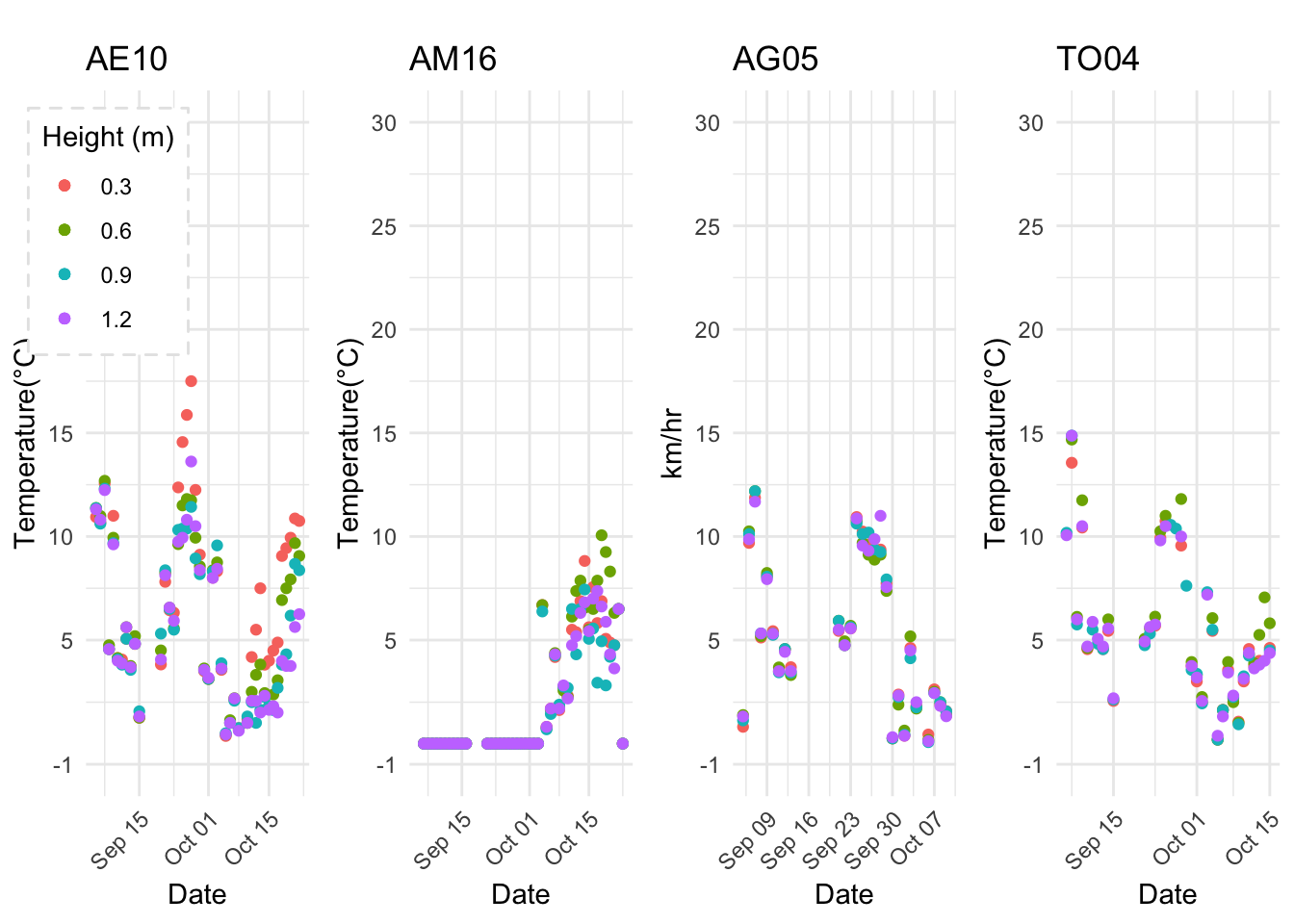
Diel variation by height (dots)
mw1 <- mclim_AE10_CN01_2018 %>% filter(month %in% c(9,10) & time > date('2018-09-05')) %>%
dplyr::group_by(month,day) %>%
dplyr::summarise(mtpoint3 = max(temp4) - min(temp4),
mtpoint6 = max(temp3) - min(temp3),
mtpoint9 = max(temp2) - min(temp2),
mtpoint12 = max(temp1) - min(temp1)) %>%
mutate(md = as.POSIXct( paste(month,day,sep = '-') , format = "%m-%d")) %>%
ggplot() +
geom_point( aes(md,mtpoint3,color = '0.3')) +
geom_point( aes(md,mtpoint6,color = '0.6')) +
geom_point( aes(md,mtpoint9,color = '0.9')) +
geom_point( aes(md,mtpoint12,color = '1.2')) +
theme_minimal() +
theme(legend.position = c(.1,.8),
legend.background = element_rect(color = "grey90",
size = .5, linetype = "dashed"),
axis.text.x=element_text(angle=45, hjust=1)) +
theme(strip.text.x = element_text(face="bold", size=12)) +
theme(strip.text.y = element_text(face="bold", size=12)) +
scale_y_continuous(limits = c(-1,30 ),breaks = c(-1,5,10,15,20,25,30)) +
labs(title="AE10",x="Date", y="Temperature(°C)", tag="", colour = "Height (m)")
mw2 <- mclim_AM16_CN01_2018 %>% filter(month %in% c(9,10) & time > date('2018-09-05')) %>%
dplyr::group_by(month,day) %>%
dplyr::summarise(mtpoint3 = max(temp4) - min(temp4),
mtpoint6 = max(temp3) - min(temp3),
mtpoint9 = max(temp2) - min(temp2),
mtpoint12 = max(temp1) - min(temp1)) %>%
mutate(md = as.POSIXct( paste(month,day,sep = '-') , format = "%m-%d")) %>%
ggplot() +
geom_point( aes(md,mtpoint3,color = '0.3')) +
geom_point( aes(md,mtpoint6,color = '0.6')) +
geom_point( aes(md,mtpoint9,color = '0.9')) +
geom_point( aes(md,mtpoint12,color = '1.2')) +
theme_minimal() +
theme(legend.position="none",
legend.background = element_rect(color = "grey90",
size = .5, linetype = "dashed"),
axis.text.x=element_text(angle=45, hjust=1)) +
theme(strip.text.x = element_text(face="bold", size=12)) +
theme(strip.text.y = element_text(face="bold", size=12)) +
scale_y_continuous(limits = c(-1,30 ),breaks = c(-1,5,10,15,20,25,30)) +
labs(title="AM16",x="Date", y="Temperature(°C)", tag="", colour = "Height (m)")
mw3 <- mclim_AG05_CN01_2018 %>% filter(month %in% c(9,10) & time > date('2018-09-05')) %>%
dplyr::group_by(month,day) %>%
dplyr::summarise(mtpoint3 = max(temp4) - min(temp4),
mtpoint6 = max(temp3) - min(temp3),
mtpoint9 = max(temp2) - min(temp2),
mtpoint12 = max(temp1) - min(temp1)) %>%
mutate(md = as.POSIXct( paste(month,day,sep = '-') , format = "%m-%d")) %>%
ggplot() +
geom_point( aes(md,mtpoint3,color = '0.3')) +
geom_point( aes(md,mtpoint6,color = '0.6')) +
geom_point( aes(md,mtpoint9,color = '0.9')) +
geom_point( aes(md,mtpoint12,color = '1.2')) +
theme_minimal() +
ylim(0,4) +
theme(legend.position="none",
legend.background = element_rect(color = "grey90",
size = .5, linetype = "dashed"),
axis.text.x=element_text(angle=45, hjust=1)) +
theme(strip.text.x = element_text(face="bold", size=12)) +
theme(strip.text.y = element_text(face="bold", size=12)) +
scale_y_continuous(limits = c(-1,30 ),breaks = c(-1,5,10,15,20,25,30)) +
labs(title="AG05",x="Date", y="km/hr", tag="", colour = "Height (m)")## Scale for 'y' is already present. Adding another scale for 'y', which
## will replace the existing scale. mw4 <- mclim_TO04_CN01_2018 %>% filter(month %in% c(9,10) & time > date('2018-09-05')) %>%
dplyr::group_by(month,day) %>%
dplyr::summarise(mtpoint3 = max(temp4) - min(temp4),
mtpoint6 = max(temp3) - min(temp3),
mtpoint9 = max(temp2) - min(temp2),
mtpoint12 = max(temp1) - min(temp1)) %>%
mutate(md = as.POSIXct( paste(month,day,sep = '-') , format = "%m-%d")) %>%
ggplot() +
geom_point( aes(md,mtpoint3,color = '0.3')) +
geom_point( aes(md,mtpoint6,color = '0.6')) +
geom_point( aes(md,mtpoint9,color = '0.9')) +
geom_point( aes(md,mtpoint12,color = '1.2')) +
theme_minimal() +
theme(legend.position="none",
legend.background = element_rect(color = "grey90",
size = .5, linetype = "dashed"),
axis.text.x=element_text(angle=45, hjust=1)) +
theme(strip.text.x = element_text(face="bold", size=12)) +
theme(strip.text.y = element_text(face="bold", size=12)) +
scale_y_continuous(limits = c(-1,30 ),breaks = c(-1,5,10,15,20,25,30)) +
labs(title="TO04",x="Date", y="Temperature(°C)", tag="", colour = "Height (m)")
library(cowplot)
main_row_temp_ts <- plot_grid(mw1,mw2,mw3,mw4, align = "v", nrow = 1)
plot_grid(main_row_temp_ts ,nrow = 1)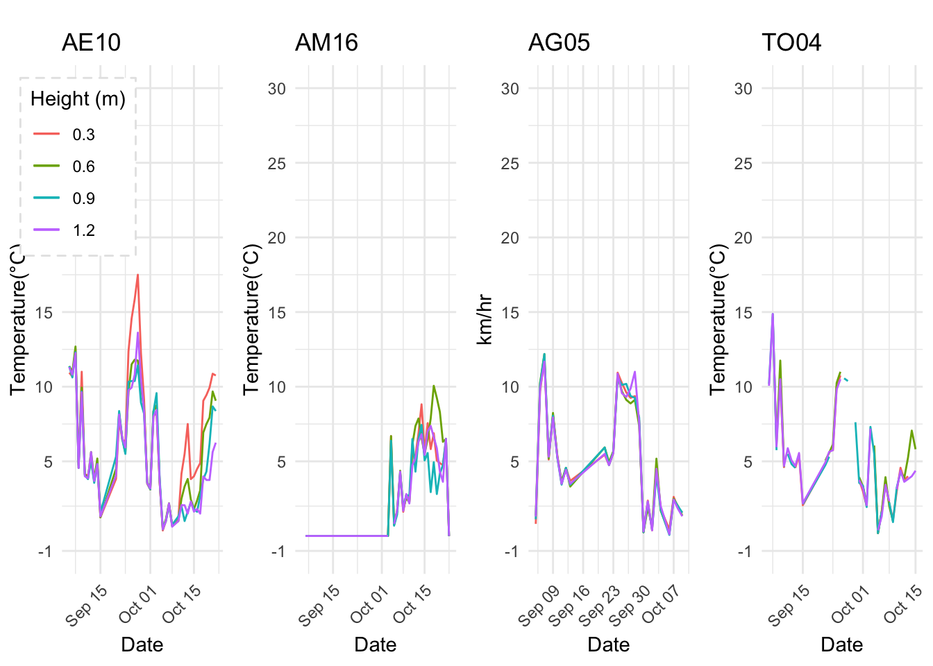
Add lines
mw1 <- mclim_AE10_CN01_2018 %>% filter(month %in% c(9,10) & time > date('2018-09-05')) %>%
dplyr::group_by(month,day) %>%
dplyr::summarise(mtpoint3 = max(temp4) - min(temp4),
mtpoint6 = max(temp3) - min(temp3),
mtpoint9 = max(temp2) - min(temp2),
mtpoint12 = max(temp1) - min(temp1)) %>%
mutate(md = as.POSIXct( paste(month,day,sep = '-') , format = "%m-%d")) %>%
ggplot() +
geom_line( aes(md,mtpoint3,color = '0.3')) +
geom_line( aes(md,mtpoint6,color = '0.6')) +
geom_line( aes(md,mtpoint9,color = '0.9')) +
geom_line( aes(md,mtpoint12,color = '1.2')) +
theme_minimal() +
theme(legend.position = c(.1,.8),
legend.background = element_rect(color = "grey90",
size = .5, linetype = "dashed"),
axis.text.x=element_text(angle=45, hjust=1)) +
theme(strip.text.x = element_text(face="bold", size=12)) +
theme(strip.text.y = element_text(face="bold", size=12)) +
scale_y_continuous(limits = c(-1,30 ),breaks = c(-1,5,10,15,20,25,30)) +
labs(title="AE10",x="Date", y="Temperature(°C)", tag="", colour = "Height (m)")
mw2 <- mclim_AM16_CN01_2018 %>% filter(month %in% c(9,10) & time > date('2018-09-05')) %>%
dplyr::group_by(month,day) %>%
dplyr::summarise(mtpoint3 = max(temp4) - min(temp4),
mtpoint6 = max(temp3) - min(temp3),
mtpoint9 = max(temp2) - min(temp2),
mtpoint12 = max(temp1) - min(temp1)) %>%
mutate(md = as.POSIXct( paste(month,day,sep = '-') , format = "%m-%d")) %>%
ggplot() +
geom_line( aes(md,mtpoint3,color = '0.3')) +
geom_line( aes(md,mtpoint6,color = '0.6')) +
geom_line( aes(md,mtpoint9,color = '0.9')) +
geom_line( aes(md,mtpoint12,color = '1.2')) +
theme_minimal() +
theme(legend.position="none",
legend.background = element_rect(color = "grey90",
size = .5, linetype = "dashed"),
axis.text.x=element_text(angle=45, hjust=1)) +
theme(strip.text.x = element_text(face="bold", size=12)) +
theme(strip.text.y = element_text(face="bold", size=12)) +
scale_y_continuous(limits = c(-1,30 ),breaks = c(-1,5,10,15,20,25,30)) +
labs(title="AM16",x="Date", y="Temperature(°C)", tag="", colour = "Height (m)")
mw3 <- mclim_AG05_CN01_2018 %>% filter(month %in% c(9,10) & time > date('2018-09-05')) %>%
dplyr::group_by(month,day) %>%
dplyr::summarise(mtpoint3 = max(temp4) - min(temp4),
mtpoint6 = max(temp3) - min(temp3),
mtpoint9 = max(temp2) - min(temp2),
mtpoint12 = max(temp1) - min(temp1)) %>%
mutate(md = as.POSIXct( paste(month,day,sep = '-') , format = "%m-%d")) %>%
ggplot() +
geom_line( aes(md,mtpoint3,color = '0.3')) +
geom_line( aes(md,mtpoint6,color = '0.6')) +
geom_line( aes(md,mtpoint9,color = '0.9')) +
geom_line( aes(md,mtpoint12,color = '1.2')) +
theme_minimal() +
ylim(0,4) +
theme(legend.position="none",
legend.background = element_rect(color = "grey90",
size = .5, linetype = "dashed"),
axis.text.x=element_text(angle=45, hjust=1)) +
theme(strip.text.x = element_text(face="bold", size=12)) +
theme(strip.text.y = element_text(face="bold", size=12)) +
scale_y_continuous(limits = c(-1,30 ),breaks = c(-1,5,10,15,20,25,30)) +
labs(title="AG05",x="Date", y="km/hr", tag="", colour = "Height (m)")## Scale for 'y' is already present. Adding another scale for 'y', which
## will replace the existing scale. mw4 <- mclim_TO04_CN01_2018 %>% filter(month %in% c(9,10) & time > date('2018-09-05')) %>%
dplyr::group_by(month,day) %>%
dplyr::summarise(mtpoint3 = max(temp4) - min(temp4),
mtpoint6 = max(temp3) - min(temp3),
mtpoint9 = max(temp2) - min(temp2),
mtpoint12 = max(temp1) - min(temp1)) %>%
mutate(md = as.POSIXct( paste(month,day,sep = '-') , format = "%m-%d")) %>%
ggplot() +
geom_line( aes(md,mtpoint3,color = '0.3')) +
geom_line( aes(md,mtpoint6,color = '0.6')) +
geom_line( aes(md,mtpoint9,color = '0.9')) +
geom_line( aes(md,mtpoint12,color = '1.2')) +
theme_minimal() +
theme(legend.position="none",
legend.background = element_rect(color = "grey90",
size = .5, linetype = "dashed"),
axis.text.x=element_text(angle=45, hjust=1)) +
theme(strip.text.x = element_text(face="bold", size=12)) +
theme(strip.text.y = element_text(face="bold", size=12)) +
scale_y_continuous(limits = c(-1,30 ),breaks = c(-1,5,10,15,20,25,30)) +
labs(title="TO04",x="Date", y="Temperature(°C)", tag="", colour = "Height (m)")
library(cowplot)
main_row_temp_ts <- plot_grid(mw1,mw2,mw3,mw4, align = "v", nrow = 1)
plot_grid(main_row_temp_ts ,nrow = 1)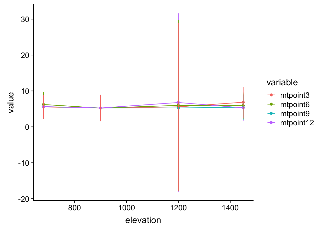
Quantify it elevation with
mw11 <- mclim_AE10_CN01_2018 %>% filter(month %in% c(9,10) & time > date('2018-09-05')) %>%
dplyr::group_by(month,day) %>%
dplyr::summarise(mtpoint3 = max(temp4) - min(temp4),
mtpoint6 = max(temp3) - min(temp3),
mtpoint9 = max(temp2) - min(temp2),
mtpoint12 = max(temp1) - min(temp1)) %>%
mutate(md = as.POSIXct( paste(month,day,sep = '-') , format = "%m-%d")) %>%
mutate(elevation = 1450 ) %>%
dplyr::select(c('mtpoint3','mtpoint6','mtpoint9','mtpoint12','elevation')) %>% as.data.frame()## Adding missing grouping variables: `month` mw21 <- mclim_AM16_CN01_2018 %>% filter(month %in% c(9,10) & time > date('2018-09-05')) %>%
dplyr::group_by(month,day) %>%
dplyr::summarise(mtpoint3 = max(temp4) - min(temp4),
mtpoint6 = max(temp3) - min(temp3),
mtpoint9 = max(temp2) - min(temp2),
mtpoint12 = max(temp1) - min(temp1)) %>%
mutate(md = as.POSIXct( paste(month,day,sep = '-') , format = "%m-%d")) %>%
mutate(elevation = 1200 ) %>%
dplyr::select(c('mtpoint3','mtpoint6','mtpoint9','mtpoint12','elevation')) %>% as.data.frame()## Adding missing grouping variables: `month` mw31 <- mclim_AG05_CN01_2018 %>% filter(month %in% c(9,10) & time > date('2018-09-05')) %>%
dplyr::group_by(month,day) %>%
dplyr::summarise(mtpoint3 = max(temp4) - min(temp4),
mtpoint6 = max(temp3) - min(temp3),
mtpoint9 = max(temp2) - min(temp2),
mtpoint12 = max(temp1) - min(temp1)) %>%
mutate(md = as.POSIXct( paste(month,day,sep = '-') , format = "%m-%d")) %>%
mutate(elevation = 900 ) %>%
dplyr::select(c('mtpoint3','mtpoint6','mtpoint9','mtpoint12','elevation')) %>% as.data.frame()## Adding missing grouping variables: `month` mw41 <- mclim_TO04_CN01_2018 %>% filter(month %in% c(9,10) & time > date('2018-09-05')) %>%
dplyr::group_by(month,day) %>% filter(temp4 != -127 &
temp1 != -127 &
temp3 != -127 &
temp2 != -127) %>%
dplyr::summarise(mtpoint3 = max(temp4) - min(temp4),
mtpoint6 = max(temp3) - min(temp3),
mtpoint9 = max(temp2) - min(temp2),
mtpoint12 = max(temp1) - min(temp1)) %>%
mutate(md = as.POSIXct( paste(month,day,sep = '-') , format = "%m-%d")) %>%
mutate(elevation = 680 ) %>%
dplyr::select(c('mtpoint3','mtpoint6','mtpoint9','mtpoint12','elevation')) %>% as.data.frame()## Adding missing grouping variables: `month` mwdveleva <- rbind(mw11,mw21,mw31,mw41)
library(reshape2)##
## Attaching package: 'reshape2'
##
## The following object is masked from 'package:tidyr':
##
## smiths mwdvelevamd <- melt(mwdveleva, id.vars = c("month", "elevation"))
data_summary <- function(data, varname, groupnames){
require(plyr)
summary_func <- function(x, col){
c(mean = mean(x[[col]], na.rm=TRUE),
sd = sd(x[[col]], na.rm=TRUE))
}
data_sum<-ddply(data, groupnames, .fun=summary_func,
varname)
data_sum <- rename(data_sum, c("mean" = varname))
return(data_sum)
}
df2 <- data_summary(mwdvelevamd, varname="value",
groupnames=c("variable", "elevation"))## Loading required package: plyr
## -------------------------------------------------------------------------
## You have loaded plyr after dplyr - this is likely to cause problems.
## If you need functions from both plyr and dplyr, please load plyr first, then dplyr:
## library(plyr); library(dplyr)
## -------------------------------------------------------------------------
##
## Attaching package: 'plyr'
##
## The following object is masked from 'package:ggpubr':
##
## mutate
##
## The following objects are masked from 'package:plotly':
##
## arrange, mutate, rename, summarise
##
## The following object is masked from 'package:lubridate':
##
## here
##
## The following objects are masked from 'package:dplyr':
##
## arrange, count, desc, failwith, id, mutate, rename, summarise,
## summarize
##
## The following object is masked from 'package:purrr':
##
## compact p<- ggplot(df2, aes(x=elevation, y=value, group=variable, color=variable)) +
geom_line() +
geom_point()+
geom_errorbar(aes(ymin=value-sd, ymax=value+sd), width=.2,
position=position_dodge(0.05))
print(p)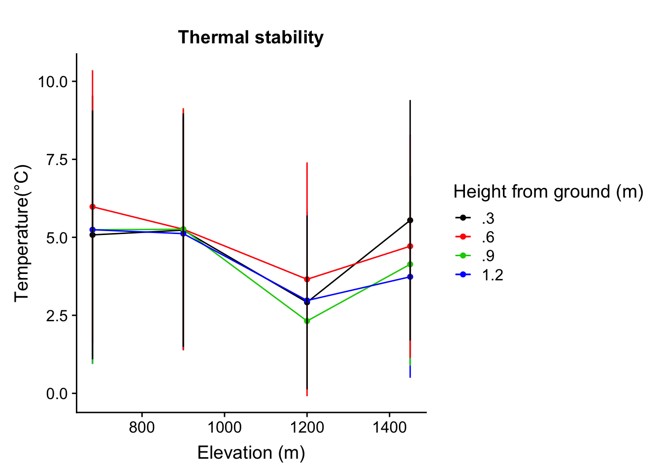
TO elevation looks funny, lets do selective days
mw11 <- mclim_AE10_CN01_2018 %>% filter(month %in% c(9,10) & time > date('2018-09-05')) %>%
dplyr::filter(day %in% c(15:20,c(7:10))) %>%
dplyr::group_by(month,day) %>%
dplyr::summarise(mtpoint3 = max(temp4) - min(temp4),
mtpoint6 = max(temp3) - min(temp3),
mtpoint9 = max(temp2) - min(temp2),
mtpoint12 = max(temp1) - min(temp1)) %>%
mutate(md = as.POSIXct( paste(month,day,sep = '-') , format = "%m-%d")) %>%
mutate(elevation = 1450 ) %>%
dplyr::select(c('mtpoint3','mtpoint6','mtpoint9','mtpoint12','elevation')) %>% as.data.frame()## Adding missing grouping variables: `month` mw21 <- mclim_AM16_CN01_2018 %>% filter(month %in% c(9,10) & time > date('2018-09-05')) %>%
dplyr::filter(day %in% c(15:20,c(7:10))) %>%
dplyr::group_by(month,day) %>%
dplyr::summarise(mtpoint3 = max(temp4) - min(temp4),
mtpoint6 = max(temp3) - min(temp3),
mtpoint9 = max(temp2) - min(temp2),
mtpoint12 = max(temp1) - min(temp1)) %>%
mutate(md = as.POSIXct( paste(month,day,sep = '-') , format = "%m-%d")) %>%
mutate(elevation = 1200 ) %>%
dplyr::select(c('mtpoint3','mtpoint6','mtpoint9','mtpoint12','elevation')) %>% as.data.frame()## Adding missing grouping variables: `month` mw31 <- mclim_AG05_CN01_2018 %>% filter(month %in% c(9,10) & time > date('2018-09-05')) %>%
dplyr::filter(day %in% c(15:20,c(7:10))) %>%
dplyr::group_by(month,day) %>%
dplyr::summarise(mtpoint3 = max(temp4) - min(temp4),
mtpoint6 = max(temp3) - min(temp3),
mtpoint9 = max(temp2) - min(temp2),
mtpoint12 = max(temp1) - min(temp1)) %>%
mutate(md = as.POSIXct( paste(month,day,sep = '-') , format = "%m-%d")) %>%
mutate(elevation = 900 ) %>%
dplyr::select(c('mtpoint3','mtpoint6','mtpoint9','mtpoint12','elevation')) %>% as.data.frame()## Adding missing grouping variables: `month` mw41 <- mclim_TO04_CN01_2018 %>% filter(month %in% c(9,10) & time > date('2018-09-05')) %>%
dplyr::filter(day %in% c(15:20,c(7:10))) %>% filter(temp4 != -127 &
temp1 != -127 &
temp3 != -127 &
temp2 != -127) %>%
dplyr::group_by(month,day) %>%
dplyr::summarise(mtpoint3 = max(temp4,na.rm = TRUE) - min(temp4,na.rm = TRUE),
mtpoint6 = max(temp3,na.rm = TRUE) - min(temp3,na.rm = TRUE),
mtpoint9 = max(temp2,na.rm = TRUE) - min(temp2,na.rm = TRUE),
mtpoint12 = max(temp1,na.rm = TRUE) - min(temp1,na.rm = TRUE)) %>%
mutate(md = as.POSIXct( paste(month,day,sep = '-') , format = "%m-%d")) %>%
mutate(elevation = 680 ) %>%
dplyr::select(c('mtpoint3','mtpoint6','mtpoint9','mtpoint12','elevation')) %>% as.data.frame()## Adding missing grouping variables: `month` mwdveleva <- rbind(mw11,mw21,mw31,mw41)
library(reshape2)
mwdvelevamd <- melt(mwdveleva, id.vars = c("month", "elevation"))
data_summary <- function(data, varname, groupnames){
require(plyr)
summary_func <- function(x, col){
c(mean = mean(x[[col]], na.rm=TRUE),
sd = sd(x[[col]], na.rm=TRUE))
}
data_sum<-ddply(data, groupnames, .fun=summary_func,
varname)
data_sum <- rename(data_sum, c("mean" = varname))
return(data_sum)
}
df2 <- data_summary(mwdvelevamd, varname="value",
groupnames=c("variable", "elevation"))
p<- ggplot(df2, aes(x=elevation, y=value, group=variable, color=variable)) +
geom_line() +
geom_point()+
geom_errorbar(aes(ymin=value-sd, ymax=value+sd), width=.9,
position=position_dodge(0.05)) +
scale_color_manual("Height from ground (m)", labels = c(".3", ".6",".9","1.2"),
values=c("mtpoint3"=1,"mtpoint6"=2,"mtpoint9"=3,"mtpoint12"=4)) +
labs(title="Thermal stability",x="Elevation (m)", y="Temperature(°C)", tag="", colour = "Height (m)")
print(p)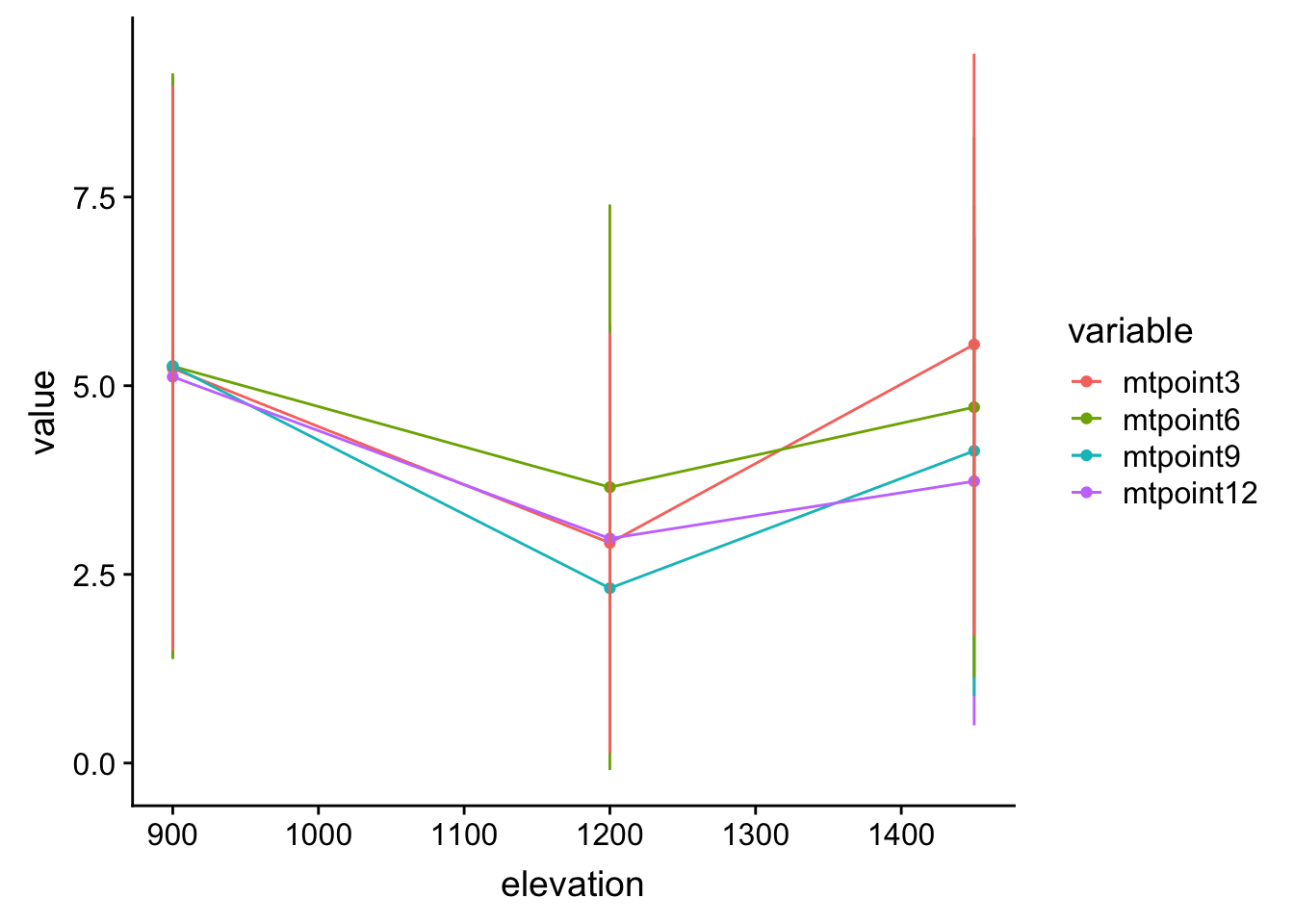
Skip first elevation and see
df2 %>%
dplyr::filter(elevation > 800) %>%
ggplot( aes(x=elevation, y=value, group=variable, color=variable)) +
geom_line() +
geom_point()+
geom_errorbar(aes(ymin=value-sd, ymax=value+sd), width=.2,
position=position_dodge(0.1))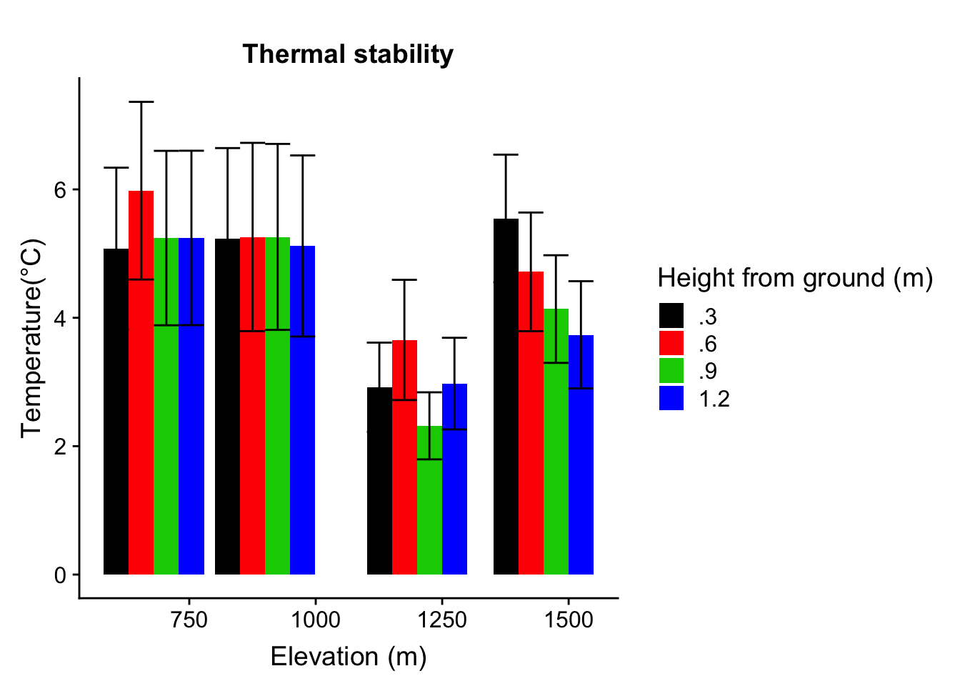
8.41 3-9-2019
Lets not calculate the SE
ggplot(mwdvelevamd, aes(elevation, value, fill=variable)) +
stat_summary(geom = "bar", fun.y = mean, position = "dodge") +
stat_summary(geom = "errorbar", fun.data = mean_se, position = "dodge") +
scale_fill_manual("Height from ground (m)", labels = c(".3", ".6",".9","1.2"),
values=c("mtpoint3"=1,"mtpoint6"=2,"mtpoint9"=3,"mtpoint12"=4)) +
labs(title="Thermal stability",x="Elevation (m)", y="Temperature(°C)", tag="", colour = "Height (m)")
pdata <- mwdvelevamd %>%
dplyr::group_by(elevation, variable) %>%
dplyr::summarise(new = list(mean_se(value))) %>%
unnest(new)
pdata %>%
ggplot(aes(elevation, y = y, fill = variable)) +
geom_col(position = "dodge") +
geom_errorbar(aes(ymin = ymin, ymax = ymax), position = "dodge") +
scale_fill_manual("Height from ground (m)", labels = c(".3", ".6",".9","1.2"),
values=c("mtpoint3"=1,"mtpoint6"=2,"mtpoint9"=3,"mtpoint12"=4) ) +
labs(title="Thermal stability",x="Elevation (m)", y="Temperature(°C)", tag="", colour = "Height (m)")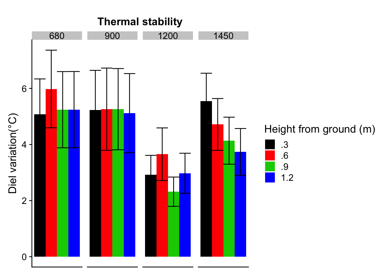
So, we agree, at least in gaps we have stability increases by height from the ground. facet_grid(. ~ day, scales = “free”)
levels(pdata$elevation) <- c("680m", "900m", "1200m","1450m")
pdata %>%
ggplot(aes(elevation, y = y, fill = variable)) +
geom_col(position = "dodge") +
geom_errorbar(aes(ymin = ymin, ymax = ymax), position = "dodge") +
facet_grid(. ~ elevation, scales = "free") +
scale_fill_manual("Height above ground (m)", labels = c(".3", ".6",".9","1.2"),
values=c("mtpoint3"=1,"mtpoint6"=2,"mtpoint9"=3,"mtpoint12"=4) ) +
labs(title="",x="Elevation (m)", y="Diurnal variation (°C)", tag="", colour = "Height (m)") +
theme_minimal(base_size=24) +
theme(axis.title.x=element_blank(),
axis.text.x=element_blank(),
axis.ticks.x=element_blank())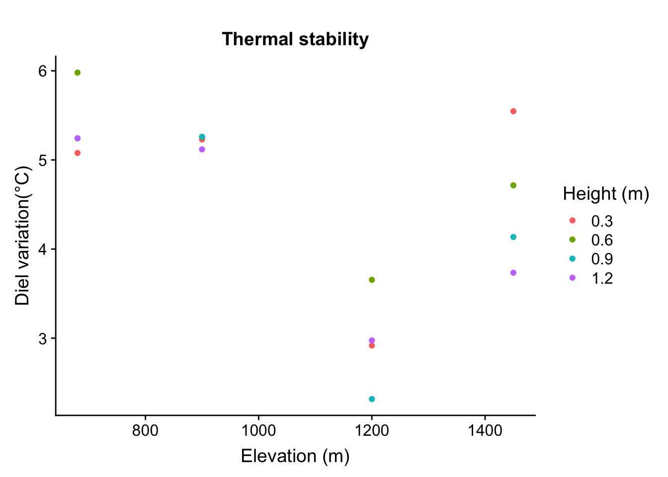
ggsave("chap1_elevation_dv.png",dpi=300, dev='png', height=8, width=8, units="in")8.42 3-10-2019
Could we explore if there is alinear relationship, why ? because temp and elevation has a linear relationship
dpata <- pdata
dpata$height <- 0
dpata[dpata$variable=='mtpoint3',]$height<- 0.3
dpata[dpata$variable=='mtpoint6',]$height<- 0.6
dpata[dpata$variable=='mtpoint9',]$height = 0.9
dpata[dpata$variable=='mtpoint12',]$height = 1.2
reg <- lm(y ~ elevation + height,data=dpata)
summary(reg)##
## Call:
## lm(formula = y ~ elevation + height, data = dpata)
##
## Residuals:
## Min 1Q Median 3Q Max
## -1.8394 -0.5185 0.2689 0.5435 1.4804
##
## Coefficients:
## Estimate Std. Error t value Pr(>|t|)
## (Intercept) 7.0309504 1.0545024 6.668 1.55e-05 ***
## elevation -0.0019109 0.0008257 -2.314 0.0377 *
## height -0.6461513 0.7195237 -0.898 0.3855
## ---
## Signif. codes: 0 '***' 0.001 '**' 0.01 '*' 0.05 '.' 0.1 ' ' 1
##
## Residual standard error: 0.9653 on 13 degrees of freedom
## Multiple R-squared: 0.3216, Adjusted R-squared: 0.2172
## F-statistic: 3.081 on 2 and 13 DF, p-value: 0.08031So, looks like my prediction is supported, only partially, the elevation does seem to influence diel variation , it makes sense, less vegetation ? or more so, change in the understory cover ?
Lets visualize the plot
dpata %>% ggplot(aes(elevation,y,color=as.factor(height))) + geom_point() +
labs(title="Thermal stability",x="Elevation (m)", y="Diel variation(°C)", tag="", colour = "Height (m)")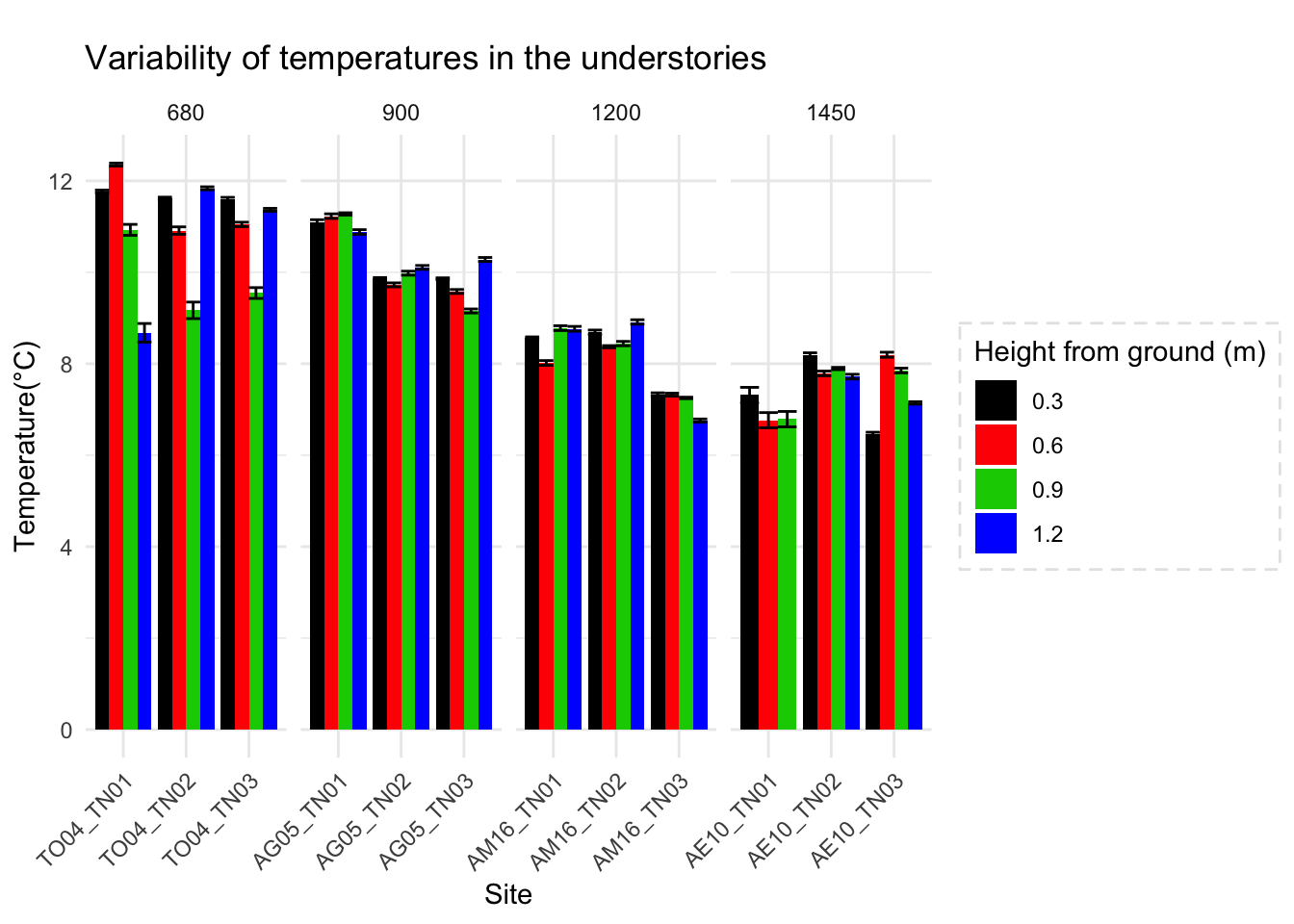
8.43 3-12-2019
Gap and Non- gap analysis
#Combine all the nodes
All_sites <- rbind(mclim_AE10_2018_ZTemp,
mclim_AG05_2018_ZTemp,
mclim_AM16_2018_ZTemp,
mclim_TO04_2018_ZTemp)
All_sites_odata <- All_sites %>%
dplyr::group_by(site, height) %>%
dplyr::summarise(new = list(mean_se(temp))) %>%
unnest(new)
All_sites_odata$elevation <- 0
All_sites_odata[All_sites_odata$site == 'TO04_TN01',]$elevation<- 680
All_sites_odata[All_sites_odata$site == 'TO04_TN02',]$elevation<- 680
All_sites_odata[All_sites_odata$site == 'TO04_TN03',]$elevation<- 680
All_sites_odata[All_sites_odata$site == 'AG05_TN01',]$elevation<- 900
All_sites_odata[All_sites_odata$site == 'AG05_TN02',]$elevation<- 900
All_sites_odata[All_sites_odata$site == 'AG05_TN03',]$elevation<- 900
All_sites_odata[All_sites_odata$site == 'AM16_TN01',]$elevation<- 1200
All_sites_odata[All_sites_odata$site == 'AM16_TN02',]$elevation<- 1200
All_sites_odata[All_sites_odata$site == 'AM16_TN03',]$elevation<- 1200
All_sites_odata[All_sites_odata$site == 'AE10_TN01',]$elevation<- 1450
All_sites_odata[All_sites_odata$site == 'AE10_TN02',]$elevation<- 1450
All_sites_odata[All_sites_odata$site == 'AE10_TN03',]$elevation<- 1450
All_sites_odata$site<- factor(All_sites_odata$site,
levels = c("TO04_TN01", "TO04_TN02", "TO04_TN03",
"AG05_TN01" , "AG05_TN02" ,"AG05_TN03",
"AM16_TN01", "AM16_TN02", "AM16_TN03",
"AE10_TN01", "AE10_TN02" ,"AE10_TN03"
))
All_sites_odata %>% mutate(hc = as.factor(height)) %>%
dplyr::filter(height > 0) %>%
dplyr::filter(y > -20) %>%
ggplot(aes(site, y = y, fill = hc)) +
geom_col(position = "dodge") +
facet_grid(. ~ elevation, scales = "free") +
theme_minimal() +
theme(
legend.background = element_rect(color = "grey90",
size = .5, linetype = "dashed"),
axis.text.x=element_text(angle=45, hjust=1)) +
geom_errorbar(aes(ymin = ymin, ymax = ymax), position = "dodge") +
scale_fill_manual("Height from ground (m)", labels = c("0.3", "0.6","0.9","1.2"),
values=c("0.3"=1,"0.6"=2,"0.9"=3,"1.2"=4) ) +
labs(title="Variability of temperatures in the understories",x="Site", y="Temperature(°C)", tag="", colour = "Height (m)")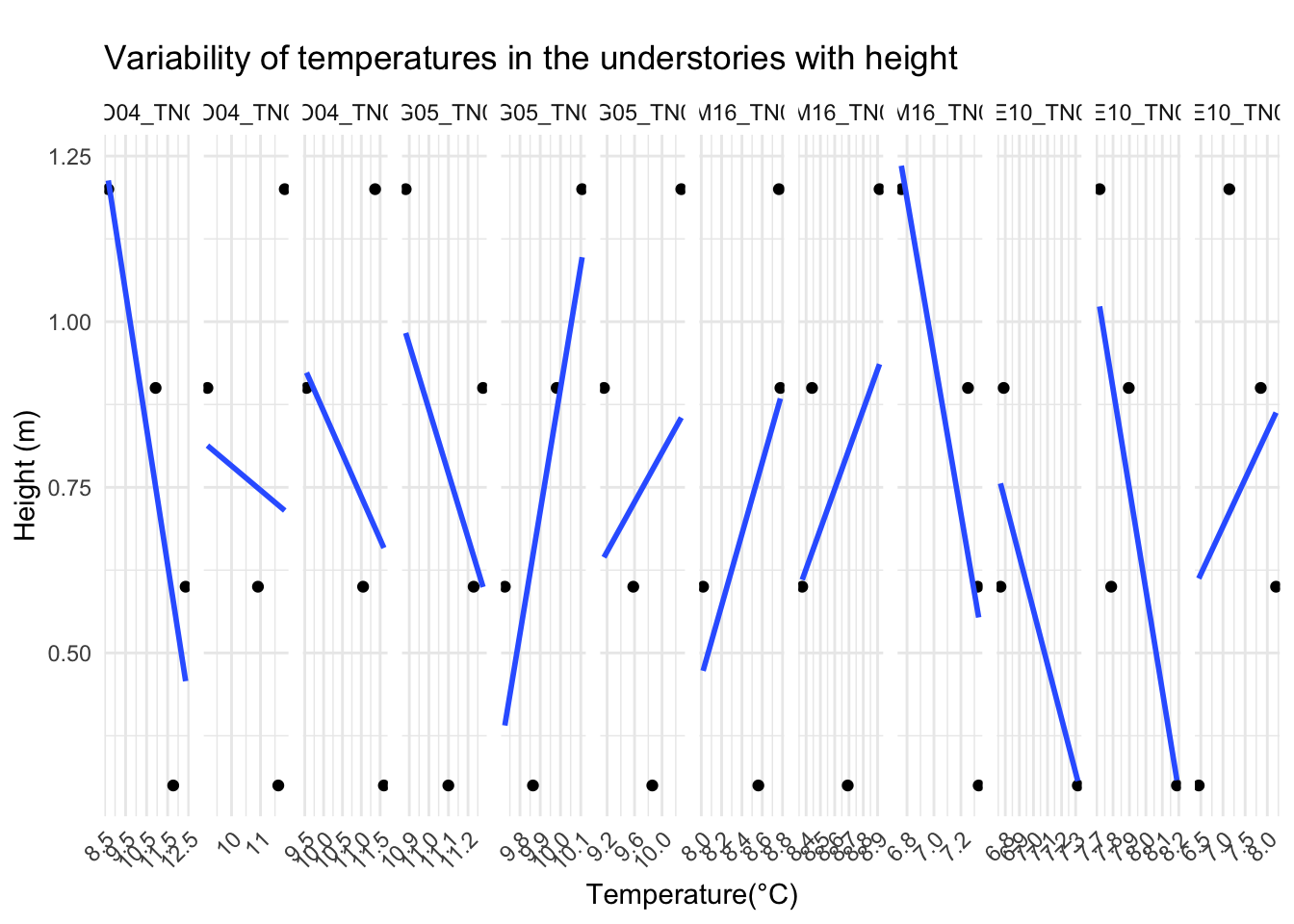
Alternate, explore how it varies with in a site
All_sites_odata %>% mutate(hc = log(height)) %>%
dplyr::filter(height > 0) %>%
dplyr::filter(y > -20) %>%
ggplot(aes(x=y, y = height)) +
geom_point() +
geom_smooth(method = 'lm', se = FALSE) +
facet_grid(. ~ site, scales = "free") +
theme_minimal() +
theme(
legend.background = element_rect(color = "grey90",
size = .5, linetype = "dashed"),
axis.text.x=element_text(angle=45, hjust=1)) +
labs(title="Variability of temperatures in the understories with height",y="Height (m)", x="Temperature(°C)", tag="", colour = "")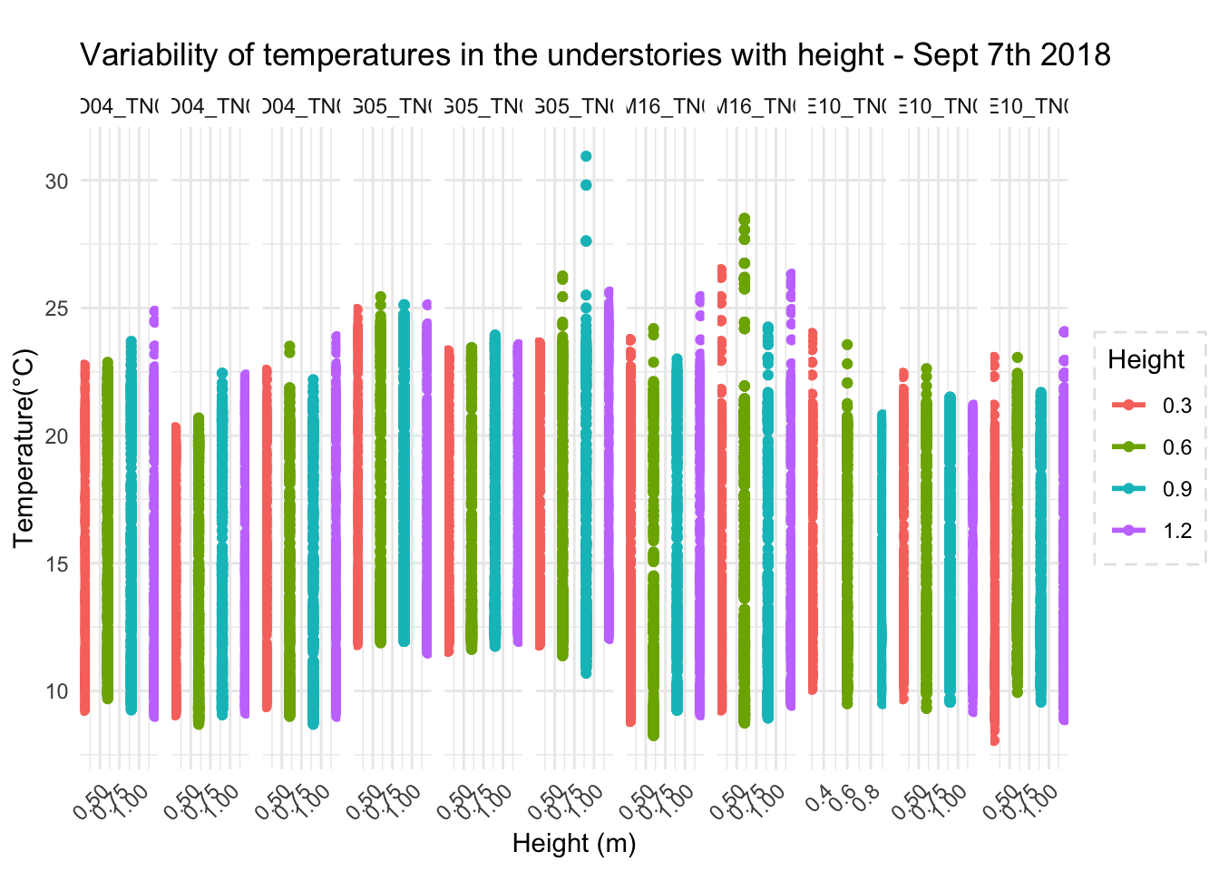 Maybe what we need is pure profiles of day and night
Day - inversion, Night -lapse
Lets look at one dayfirst
All_sites$site<- factor(All_sites$site,
levels = c("TO04_TN01", "TO04_TN02", "TO04_TN03",
"AG05_TN01" , "AG05_TN02" ,"AG05_TN03",
"AM16_TN01", "AM16_TN02", "AM16_TN03",
"AE10_TN01", "AE10_TN02" ,"AE10_TN03"
))
All_sites %>% mutate(hc = log(height)) %>%
dplyr::filter(height > 0 & hr %in% c(1:24) & day %in% c(7) & month %in% c(9)) %>%
dplyr::filter(temp > -20) %>%
ggplot(aes(y=temp, x = height,color=factor(height))) +
geom_point() +
geom_smooth(method = 'lm', se = FALSE) +
facet_grid(. ~ site, scales = "free") +
theme_minimal() +
theme(
legend.background = element_rect(color = "grey90",
size = .5, linetype = "dashed"),
axis.text.x=element_text(angle=45, hjust=1)) +
labs(title="Variability of temperatures in the understories with height - Sept 7th 2018",x="Height (m)", y="Temperature(°C)", tag="", colour = "Height")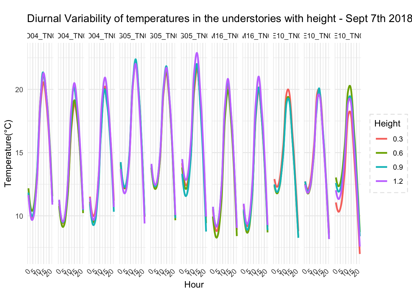
All_sites %>% mutate(hc = log(height)) %>%
dplyr::filter(height > 0 & hr %in% c(1:24) & day %in% c(7) & month %in% c(9)) %>%
dplyr::filter(temp > -20) %>%
ggplot(aes(y=temp, x = hr,color=factor(height))) +
# geom_point() +
geom_smooth(method = 'loess', se = FALSE) +
facet_grid(. ~ site, scales = "free") +
theme_minimal() +
theme(
legend.background = element_rect(color = "grey90",
size = .5, linetype = "dashed"),
axis.text.x=element_text(angle=45, hjust=1)) +
labs(title="Diurnal Variability of temperatures in the understories with height - Sept 7th 2018",x="Hour", y="Temperature(°C)", tag="", colour = "Height")
Is the vertical difference in temp significant ?
Lets visualize the plot
All_sites_odata_filter <- All_sites_odata %>% mutate(hc = as.factor(height)) %>%
dplyr::filter(height > 0) %>%
dplyr::filter(y > -20) %>% as.data.frame()
reg_all <- lm(y ~ height,data=All_sites_odata_filter)
summary(reg_all)##
## Call:
## lm(formula = y ~ height, data = All_sites_odata_filter)
##
## Residuals:
## Min 1Q Median 3Q Max
## -2.8436 -1.3134 -0.2192 1.7059 3.1144
##
## Coefficients:
## Estimate Std. Error t value Pr(>|t|)
## (Intercept) 9.3511 0.5946 15.726 <2e-16 ***
## height -0.1818 0.7326 -0.248 0.805
## ---
## Signif. codes: 0 '***' 0.001 '**' 0.01 '*' 0.05 '.' 0.1 ' ' 1
##
## Residual standard error: 1.67 on 45 degrees of freedom
## Multiple R-squared: 0.001367, Adjusted R-squared: -0.02083
## F-statistic: 0.06158 on 1 and 45 DF, p-value: 0.8051So, the difference in temp at differnt heights not signifcant
So, lets see if at two heights , is it relevant (0.3 and 1.2)
All_sites_odata_filter_height <- All_sites_odata %>% mutate(hc = as.factor(height)) %>%
dplyr::filter(height > 0 & height %in% c(0.3,1.2)) %>%
dplyr::filter(y > -20) %>% as.data.frame()
reg_all_height <- lm(y ~ height,data=All_sites_odata_filter_height)
summary(reg_all_height)##
## Call:
## lm(formula = y ~ height, data = All_sites_odata_filter_height)
##
## Residuals:
## Min 1Q Median 3Q Max
## -2.9091 -1.3841 -0.3997 1.6528 2.5243
##
## Coefficients:
## Estimate Std. Error t value Pr(>|t|)
## (Intercept) 9.37822 0.71522 13.112 1.4e-11 ***
## height -0.05403 0.83389 -0.065 0.949
## ---
## Signif. codes: 0 '***' 0.001 '**' 0.01 '*' 0.05 '.' 0.1 ' ' 1
##
## Residual standard error: 1.798 on 21 degrees of freedom
## Multiple R-squared: 0.0001999, Adjusted R-squared: -0.04741
## F-statistic: 0.004198 on 1 and 21 DF, p-value: 0.9489Look at how Gaps compare across elevations
#Combine all the nodes
All_sites_odata_canopy <- All_sites %>%
dplyr::group_by(site, canopy) %>%
dplyr::summarise(new = list(mean_se(temp))) %>%
unnest(new)
All_sites_odata_canopy$elevation <- 0
All_sites_odata_canopy[All_sites_odata_canopy$site == 'TO04_TN01',]$elevation<- 680
All_sites_odata_canopy[All_sites_odata_canopy$site == 'TO04_TN02',]$elevation<- 680
All_sites_odata_canopy[All_sites_odata_canopy$site == 'TO04_TN03',]$elevation<- 680
All_sites_odata_canopy[All_sites_odata_canopy$site == 'AG05_TN01',]$elevation<- 900
All_sites_odata_canopy[All_sites_odata_canopy$site == 'AG05_TN02',]$elevation<- 900
All_sites_odata_canopy[All_sites_odata_canopy$site == 'AG05_TN03',]$elevation<- 900
All_sites_odata_canopy[All_sites_odata_canopy$site == 'AM16_TN01',]$elevation<- 1200
All_sites_odata_canopy[All_sites_odata_canopy$site == 'AM16_TN02',]$elevation<- 1200
All_sites_odata_canopy[All_sites_odata_canopy$site == 'AM16_TN03',]$elevation<- 1200
All_sites_odata_canopy[All_sites_odata_canopy$site == 'AE10_TN01',]$elevation<- 1450
All_sites_odata_canopy[All_sites_odata_canopy$site == 'AE10_TN02',]$elevation<- 1450
All_sites_odata_canopy[All_sites_odata_canopy$site == 'AE10_TN03',]$elevation<- 1450
All_sites_odata_canopy$site<- factor(All_sites_odata_canopy$site,
levels = c("TO04_TN01", "TO04_TN02", "TO04_TN03",
"AG05_TN01" , "AG05_TN02" ,"AG05_TN03",
"AM16_TN01", "AM16_TN02", "AM16_TN03",
"AE10_TN01", "AE10_TN02" ,"AE10_TN03"
))
All_sites_odata_canopy %>%
dplyr::filter(y > -20) %>%
ggplot(aes(site, y = y, fill = canopy)) +
geom_col(position = "dodge") +
facet_grid(. ~ elevation, scales = "free") +
theme_minimal() +
theme(
legend.background = element_rect(color = "grey90",
size = .5, linetype = "dashed"),
axis.text.x=element_text(angle=45, hjust=1)) +
geom_errorbar(aes(ymin = ymin, ymax = ymax), position = "dodge") +
scale_fill_manual("Type", labels = c("Open", "Closed"),
values=c("Open"=1,"Closed"=2) ) +
labs(title="Variability of temperatures in the understories (Gap vs Non Gap)",x="Site", y="Temperature(°C)", tag="", colour = "Canopy")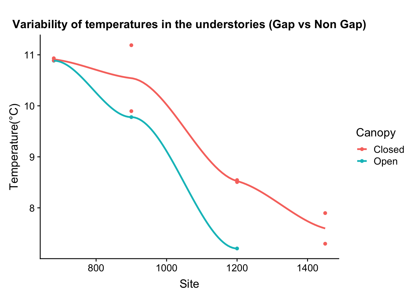
Very close, is it significant ?
All_sites_odata_canopy_filter <- All_sites_odata_canopy %>%
dplyr::filter(y > -20) %>% as.data.frame()
reg_all_canopy <- lm(y ~ elevation + canopy ,data=All_sites_odata_canopy_filter)
summary(reg_all_canopy)##
## Call:
## lm(formula = y ~ elevation + canopy, data = All_sites_odata_canopy_filter)
##
## Residuals:
## Min 1Q Median 3Q Max
## -0.7039 -0.3317 -0.1295 0.3520 0.9986
##
## Coefficients:
## Estimate Std. Error t value Pr(>|t|)
## (Intercept) 14.7380226 0.6723109 21.921 1.98e-08 ***
## elevation -0.0050539 0.0006085 -8.306 3.33e-05 ***
## canopyOpen -0.7660311 0.3813530 -2.009 0.0794 .
## ---
## Signif. codes: 0 '***' 0.001 '**' 0.01 '*' 0.05 '.' 0.1 ' ' 1
##
## Residual standard error: 0.5509 on 8 degrees of freedom
## Multiple R-squared: 0.8962, Adjusted R-squared: 0.8702
## F-statistic: 34.53 on 2 and 8 DF, p-value: 0.0001161How about changes in elevation because of canopy ?
All_sites_odata_canopy_filter <- All_sites_odata_canopy %>%
dplyr::filter(y > -20) %>% as.data.frame()
reg_all_canopy <- lm(y ~ elevation * canopy ,data=All_sites_odata_canopy_filter)
summary(reg_all_canopy)##
## Call:
## lm(formula = y ~ elevation * canopy, data = All_sites_odata_canopy_filter)
##
## Residuals:
## Min 1Q Median 3Q Max
## -0.27886 -0.22793 -0.18959 0.08614 1.06496
##
## Coefficients:
## Estimate Std. Error t value Pr(>|t|)
## (Intercept) 14.2923986 0.6536613 21.865 1.06e-07 ***
## elevation -0.0046325 0.0005958 -7.775 0.000109 ***
## canopyOpen 1.6378303 1.4271211 1.148 0.288820
## elevation:canopyOpen -0.0025346 0.0014612 -1.735 0.126392
## ---
## Signif. codes: 0 '***' 0.001 '**' 0.01 '*' 0.05 '.' 0.1 ' ' 1
##
## Residual standard error: 0.4925 on 7 degrees of freedom
## Multiple R-squared: 0.9274, Adjusted R-squared: 0.8963
## F-statistic: 29.8 on 3 and 7 DF, p-value: 0.0002332Nada
How about just canopy
All_sites_odata_canopy_filter <- All_sites_odata_canopy %>%
dplyr::filter(y > -20) %>% as.data.frame()
reg_all_canopy <- lm(y ~ canopy ,data=All_sites_odata_canopy_filter)
summary(reg_all_canopy)##
## Call:
## lm(formula = y ~ canopy, data = All_sites_odata_canopy_filter)
##
## Residuals:
## Min 1Q Median 3Q Max
## -2.0971 -1.1924 0.4897 1.5175 1.7946
##
## Coefficients:
## Estimate Std. Error t value Pr(>|t|)
## (Intercept) 9.3936 0.5696 16.491 4.94e-08 ***
## canopyOpen -0.1048 1.0908 -0.096 0.926
## ---
## Signif. codes: 0 '***' 0.001 '**' 0.01 '*' 0.05 '.' 0.1 ' ' 1
##
## Residual standard error: 1.611 on 9 degrees of freedom
## Multiple R-squared: 0.001025, Adjusted R-squared: -0.11
## F-statistic: 0.009234 on 1 and 9 DF, p-value: 0.9256 All_sites_odata_canopy %>%
dplyr::filter(y > -20) %>% ggplot() +
aes(elevation,y,color=canopy) + geom_point() +
geom_smooth(method = 'auto', se = FALSE) +
scale_color_manual("", labels = c("Dense canopy", "Gaps"),
# values=c("Open"=1,"Closed"=2) )+
values= c("green", "orange") ) +
theme_minimal(base_size=24) +
labs(title="",x="Elevation (m)", y="Mean Temperature (°C)", tag="", colour = "")## `geom_smooth()` using method = 'loess' and formula 'y ~ x'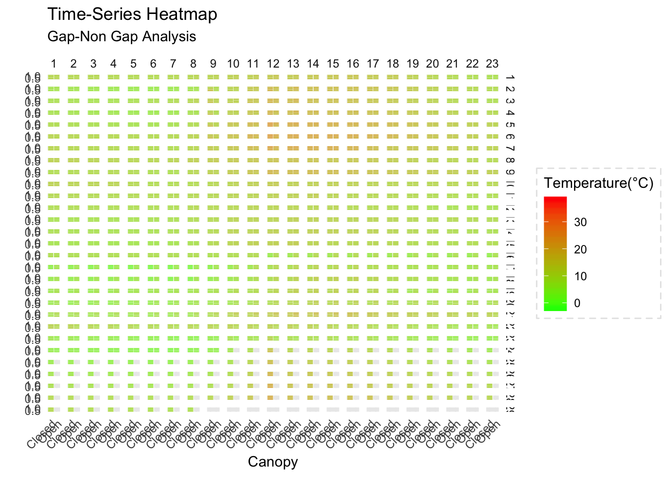
ggsave("chap1_elevation_temp.png",dpi=300, dev='png', height=7, width=8, units="in")## `geom_smooth()` using method = 'loess' and formula 'y ~ x'8.44 11-23-2019
Get the slope
allsites_gaps_only <- All_sites_odata_canopy %>%
dplyr::filter(y > -20 & canopy=="Open")
allsites_canopy_only <- All_sites_odata_canopy %>%
dplyr::filter(y > -20 & canopy=="Closed")
fit_DC <- lm(y ~ elevation, data = allsites_canopy_only)
fit_Gaps <- lm(y ~ elevation, data = allsites_gaps_only)
All_sites_odata_canopy %>%
dplyr::filter(y > -20) %>% ggplot() +
aes(elevation,y,color=canopy) + geom_point() +
geom_smooth(method = 'lm', se = FALSE) +
scale_color_manual("", labels = c("Dense canopy", "Gaps"),
# values=c("Open"=1,"Closed"=2) )+
values= c("green", "orange") ) +
theme_minimal(base_size=24) +
labs(title="",x="Elevation (m)", y="Mean Temperature (°C)", tag="", colour = "")
ggsave("chap1_elevation_temp.png",dpi=300, dev='png', height=7, width=8, units="in")Get the JL way
All_sites_odata_canopy %>%
dplyr::filter(y > -20) %>% ggplot() +
aes(y,elevation,color=canopy) + geom_point() +
geom_smooth(method = 'lm', se = FALSE) +
scale_color_manual("", labels = c("Dense canopy", "Gaps"),
# values=c("Open"=1,"Closed"=2) )+
values= c("green", "orange") ) +
theme_minimal(base_size=24) +
labs(title="",y="Elevation (m)", x="Mean Temperature (°C)", tag="", colour = "")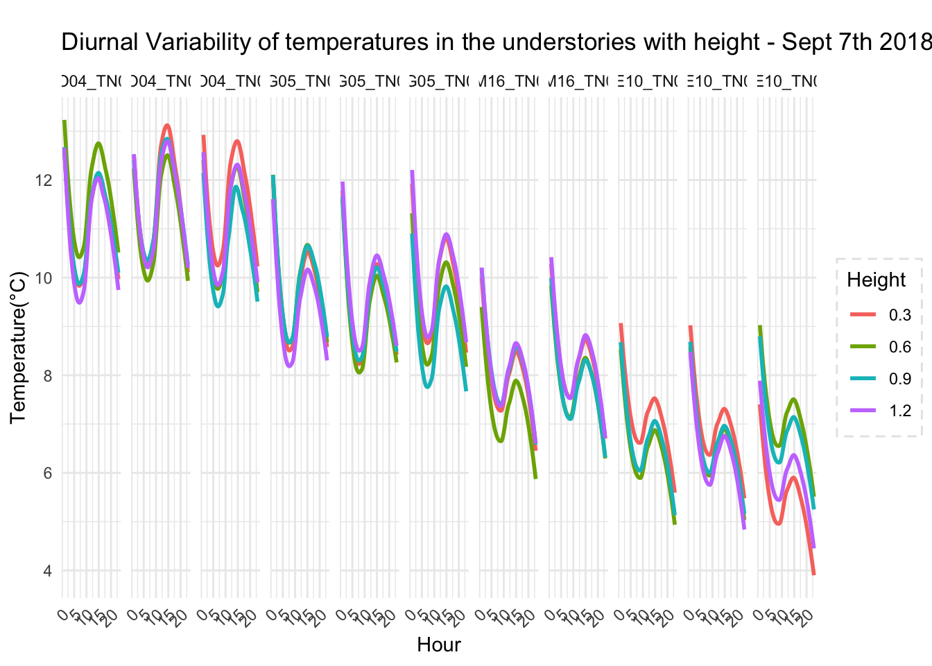
ggsave("chap1_elevation_temp.png",dpi=300, dev='png', height=7, width=8, units="in")8.45 3-21-2019
All_sites %>% mutate(hc = log(height)) %>%
dplyr::filter(height > 0 & hr %in% c(1:24) & month %in% c(9)) %>%
dplyr::filter(temp > -20) %>%
ggplot(aes(canopy, height, fill = temp)) +
geom_tile(colour = "white") +
facet_grid(day~hr) +
scale_fill_gradient(low="green", high="red") +
labs(x="Canopy",
y="",
title = "Time-Series Heatmap",
subtitle="Gap-Non Gap Analysis",
fill="Temperature(°C)") +
theme_minimal() +
theme(
legend.background = element_rect(color = "grey90",
size = .5, linetype = "dashed"),
axis.text.x=element_text(angle=45, hjust=1)) 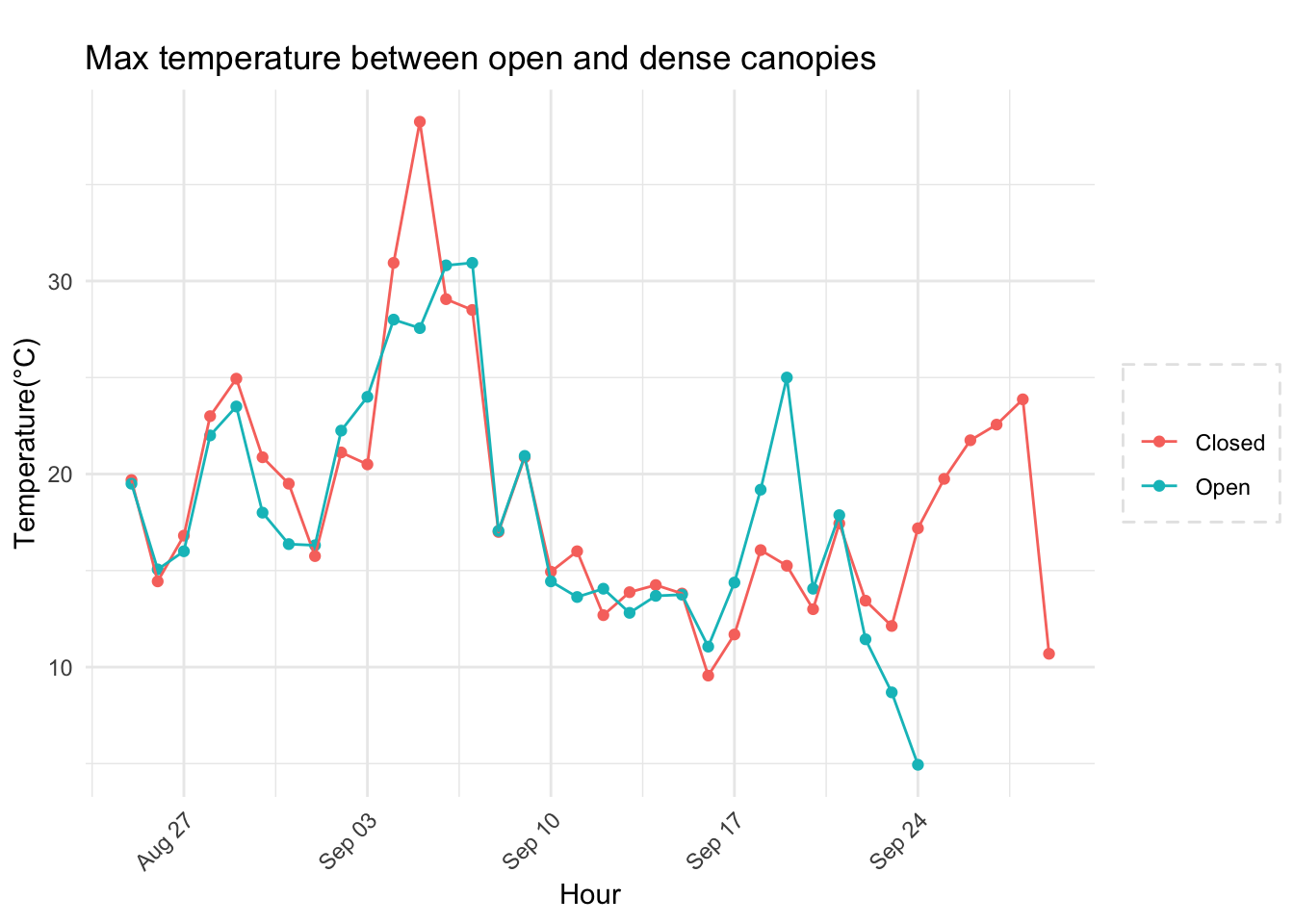
Todo - Diel temperature variation in gaps and non-gaps.
Lets look at temperature variation at
library(gganimate)##
## Attaching package: 'gganimate'## The following object is masked from 'package:raster':
##
## animatelibrary(av)
library(gifski)
animate_allsites <- All_sites %>% mutate(hc = log(height)) %>%
dplyr::filter(height > 0 & hr %in% c(1:24) & month %in% c(9)) %>%
dplyr::filter(temp > -20) %>% as.data.frame()
plot_allsites <- ggplot(animate_allsites,aes(y=temp, x = hr,color=factor(height))) +
# geom_point() +
geom_smooth(method = 'loess', se = FALSE) +
facet_grid(. ~ site, scales = "free") +
theme_minimal() +
theme(
legend.background = element_rect(color = "grey90",
size = .5, linetype = "dashed"),
axis.text.x=element_text(angle=45, hjust=1)) +
labs(title="Diurnal Variability of temperatures in the understories with height - {current_frame} Sept 2018",x="Hour", y="Temperature(°C)", tag="", colour = "Height")
anim_pp <- plot_allsites + transition_manual(day) +ease_aes('cubic-in-out') +
enter_fade() + exit_shrink()
animate(
anim_pp + enter_fade() + exit_fly(y_loc = 1),
renderer = av_renderer()
)## nframes and fps adjusted to match transitionAll_sites %>% mutate(hc = log(height)) %>%
dplyr::filter(height > 0 & hr %in% c(1:24) & day %in% c(10) & month %in% c(9)) %>%
dplyr::filter(temp > -20) %>%
ggplot(aes(y=temp, x = hr,color=factor(height))) +
# geom_point() +
geom_smooth(method = 'loess', se = FALSE) +
facet_grid(. ~ site, scales = "free") +
theme_minimal() +
theme(
legend.background = element_rect(color = "grey90",
size = .5, linetype = "dashed"),
axis.text.x=element_text(angle=45, hjust=1)) +
labs(title="Diurnal Variability of temperatures in the understories with height - Sept 7th 2018",x="Hour", y="Temperature(°C)", tag="", colour = "Height")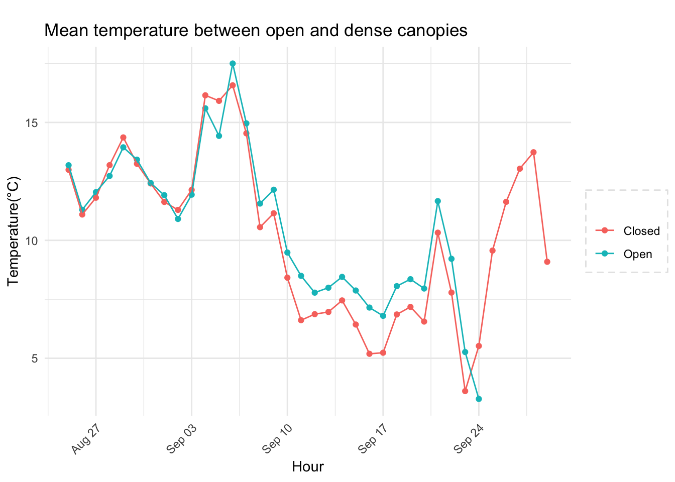 ## 5-23-2019
Max Temperatures
library(tidyverse)
All_sites %>% mutate(hc = log(height)) %>%
dplyr::filter(height > 0 & hr %in% c(1:24)) %>%
dplyr::filter(temp > -20) %>%
dplyr::group_by(canopy,month,day) %>%
dplyr::summarise(min_temp= min(temp), max_temp = max(temp), mean_temp = mean(temp)) %>%
dplyr::mutate(dt_d = lubridate::ymd(paste('2018',month,day,sep = '-'))) %>%
ggplot(aes(y=max_temp, x = dt_d ,color=canopy)) +
geom_point() +
geom_line() +
theme_minimal() +
theme(
legend.background = element_rect(color = "grey90",
size = .5, linetype = "dashed"),
axis.text.x=element_text(angle=45, hjust=1)) +
labs(title="Max temperature between open and dense canopies",x="Hour", y="Temperature(°C)", tag="", colour = "")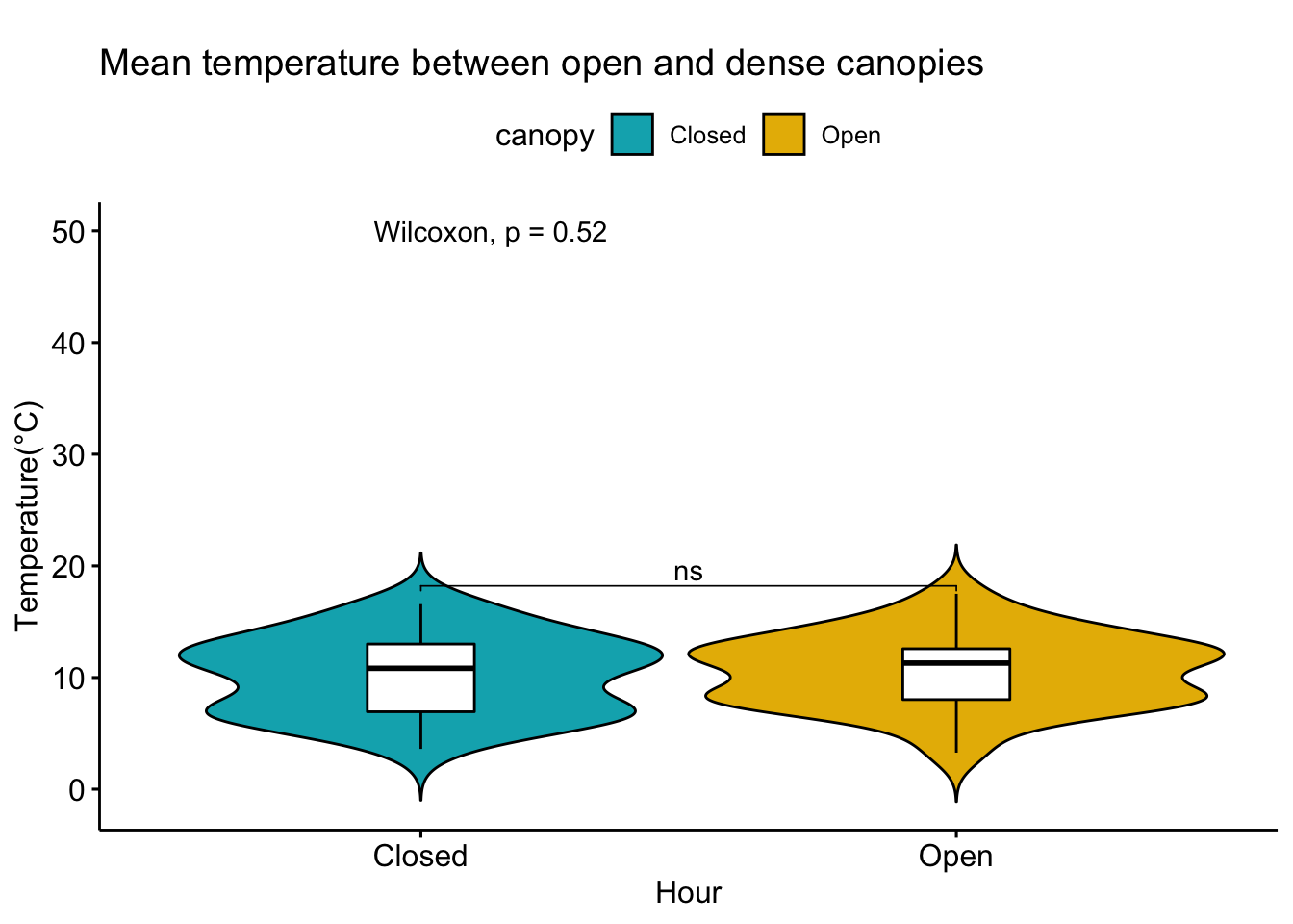 Min
Min
library(tidyverse)
All_sites %>% mutate(hc = log(height)) %>%
dplyr::filter(height > 0 & hr %in% c(1:24)) %>%
dplyr::filter(temp > -20) %>%
dplyr::group_by(canopy,month,day) %>%
dplyr::summarise(min_temp= min(temp), max_temp = max(temp), mean_temp = mean(temp)) %>%
dplyr::mutate(dt_d = lubridate::ymd(paste('2018',month,day,sep = '-'))) %>%
ggplot(aes(y=min_temp, x = dt_d ,color=canopy)) +
geom_point() +
geom_line() +
theme_minimal() +
theme(
legend.background = element_rect(color = "grey90",
size = .5, linetype = "dashed"),
axis.text.x=element_text(angle=45, hjust=1)) +
labs(title="Min temperature between open and dense canopies",x="Hour", y="Temperature(°C)", tag="", colour = "")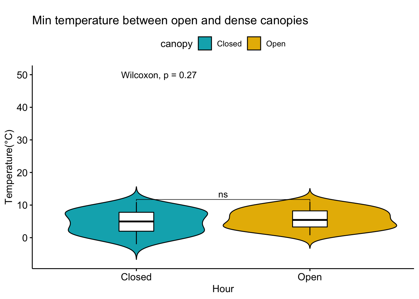 Mean
Mean
library(tidyverse)
All_sites %>% mutate(hc = log(height)) %>%
dplyr::filter(height > 0 & hr %in% c(1:24)) %>%
dplyr::filter(temp > -20) %>%
dplyr::group_by(canopy,month,day) %>%
dplyr::summarise(min_temp= min(temp), max_temp = max(temp), mean_temp = mean(temp)) %>%
dplyr::mutate(dt_d = lubridate::ymd(paste('2018',month,day,sep = '-'))) %>%
ggplot(aes(y=mean_temp, x = dt_d ,color=canopy)) +
geom_point() +
geom_line() +
theme_minimal() +
theme(
legend.background = element_rect(color = "grey90",
size = .5, linetype = "dashed"),
axis.text.x=element_text(angle=45, hjust=1)) +
labs(title="Mean temperature between open and dense canopies",x="Hour", y="Temperature(°C)", tag="", colour = "")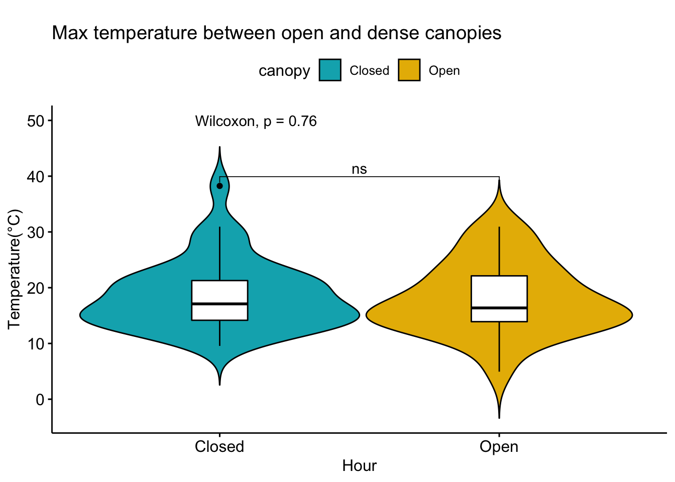
8.46 11-19-2019
Plot min and max
library(tidyverse)
All_sites %>% mutate(hc = log(height)) %>%
dplyr::filter(height > 0 & hr %in% c(1:24)) %>%
dplyr::filter(temp > -20) %>%
dplyr::group_by(canopy,month,day) %>%
dplyr::summarise(min_temp= min(temp), max_temp = max(temp), mean_temp = mean(temp)) %>%
dplyr::mutate(dt_d = lubridate::ymd(paste('2018',month,day,sep = '-'))) %>%
ggplot() +
geom_point(aes(y=min_temp, x = dt_d , color='Min')) +
geom_point(aes(y=max_temp, x = dt_d , color='Max')) +
geom_line(aes(y=min_temp, x = dt_d ,linetype=canopy)) +
geom_line(aes(y=max_temp, x = dt_d ,linetype=canopy)) +
theme_minimal() +
theme(
legend.background = element_rect(color = "grey90",
size = .5, linetype = "dashed"),
axis.text.x=element_text(angle=45, hjust=1)) +
labs(title="Min temperature between open and dense canopies",x="Hour", y="Temperature(°C)", tag="", colour = "")
8.47 11-20-2019
Plot min and max
library(tidyverse)
All_sites %>% mutate(hc = log(height)) %>%
dplyr::filter(height > 0 & hr %in% c(1:24)) %>%
dplyr::filter(temp > -20) %>%
dplyr::group_by(canopy,month,day) %>%
dplyr::summarise(min_temp= min(temp), max_temp = max(temp), mean_temp = mean(temp)) %>%
dplyr::mutate(dv= max_temp - min_temp ) %>%
dplyr::mutate(dt_d = lubridate::ymd(paste('2018',month,day,sep = '-'))) %>%
ggplot() +
geom_point(aes(y=dv, x = dt_d , color='DV')) +
geom_line(aes(y=dv, x = dt_d ,linetype=canopy)) +
theme_minimal() +
theme(
legend.background = element_rect(color = "grey90",
size = .5, linetype = "dashed"),
axis.text.x=element_text(angle=45, hjust=1)) +
labs(title="Diurnal variation between gap and dense canopies",x="Hour", y="Temperature(°C)", tag="", colour = "")
Find how the min and max is by elevation
Violin plot - With significance test
All_site_withelevation <- All_sites %>% mutate(hc = log(height)) %>%
dplyr::filter(height > 0 & hr %in% c(1:24)) %>%
dplyr::filter(temp > -20) %>% as.data.frame()
All_site_withelevation$elevation <- 0
All_site_withelevation[All_site_withelevation$site == 'TO04_TN01',]$elevation<- 680
All_site_withelevation[All_site_withelevation$site == 'TO04_TN02',]$elevation<- 680
All_site_withelevation[All_site_withelevation$site == 'TO04_TN03',]$elevation<- 680
All_site_withelevation[All_site_withelevation$site == 'AG05_TN01',]$elevation<- 900
All_site_withelevation[All_site_withelevation$site == 'AG05_TN02',]$elevation<- 900
All_site_withelevation[All_site_withelevation$site == 'AG05_TN03',]$elevation<- 900
All_site_withelevation[All_site_withelevation$site == 'AM16_TN01',]$elevation<- 1200
All_site_withelevation[All_site_withelevation$site == 'AM16_TN02',]$elevation<- 1200
#All_site_withelevation[All_site_withelevation$site == 'AM16_TN03',]$elevation<- 1200
All_site_withelevation[All_site_withelevation$site == 'AE10_TN01',]$elevation<- 1450
All_site_withelevation[All_site_withelevation$site == 'AE10_TN02',]$elevation<- 1450
All_site_withelevation[All_site_withelevation$site == 'AE10_TN03',]$elevation<- 1450library(tidyverse)
All_site_withelevation %>%
dplyr::group_by(elevation,canopy,month,day) %>%
dplyr::summarise(min_temp= min(temp), max_temp = max(temp), mean_temp = mean(temp)) %>%
dplyr::mutate(dt_d = lubridate::ymd(paste('2018',month,day,sep = '-'))) %>%
ggplot(aes(y=mean_temp, x = dt_d ,color=canopy)) +
geom_point() +
geom_line() +
facet_grid(.~elevation)+
theme_minimal() +
theme(
legend.background = element_rect(color = "grey90",
size = .5, linetype = "dashed"),
axis.text.x=element_text(angle=45, hjust=1)) +
labs(title="Mean temperature between gap and dense canopies",x="Hour", y="Temperature(°C)", tag="", colour = "")
library(ggpubr)
allsites_sigf <- All_sites %>% mutate(hc = log(height)) %>%
dplyr::filter(height > 0 & hr %in% c(1:24)) %>%
dplyr::filter(temp > -20) %>%
dplyr::group_by(canopy,month,day) %>%
dplyr::summarise(min_temp= min(temp), max_temp = max(temp), mean_temp = mean(temp)) %>%
dplyr::mutate(dv= max_temp - min_temp ) %>%
dplyr::mutate(dt_d = lubridate::ymd(paste('2018',month,day,sep = '-'))) %>% as.data.frame()
allsites_elevation_sigf <- All_site_withelevation %>% mutate(hc = log(height)) %>%
dplyr::filter(height > 0 & hr %in% c(1:24)) %>%
dplyr::filter(temp > -20) %>%
dplyr::group_by(elevation, canopy,month,day) %>%
dplyr::summarise(min_temp= min(temp), max_temp = max(temp), mean_temp = mean(temp)) %>%
dplyr::mutate(dv= max_temp - min_temp ) %>%
dplyr::mutate(dt_d = lubridate::ymd(paste('2018',month,day,sep = '-'))) %>% as.data.frame()
my_comparisons <- list( c("Closed", "Open") )
ggviolin(allsites_sigf, x = "canopy", y = "mean_temp", fill = "canopy",
palette = c("#00AFBB","#E7B800"),
add = "boxplot", add.params = list(fill = "white"))+
stat_compare_means(comparisons = my_comparisons, label = "p.signif")+ # Add significance levels
stat_compare_means(label.y = 50) +
labs(title="Mean temperature between open and dense canopies",x="Hour", y="Temperature(°C)", tag="", colour = "")
allsites_elevation_sigf %>% ggplot() +
aes(elevation,dv,color=canopy) + geom_point() +
geom_smooth(method = 'lm', se = FALSE) +
scale_color_manual("", labels = c("Dense canopy", "Gaps"),
# values=c("Open"=1,"Closed"=2) )+
values= c("green", "orange") ) +
theme_minimal(base_size=24) +
labs(title="",x="Elevation (m)", y="Mean Temperature (°C)", tag="", colour = "")
ggsave("chap1_elevation_dv.png",dpi=300, dev='png', height=7, width=8, units="in")my_comparisons <- list( c("Closed", "Open") )
ggviolin(allsites_sigf, x = "canopy", y = "min_temp", fill = "canopy",
palette = c("#00AFBB","#E7B800"),
add = "boxplot", add.params = list(fill = "white"))+
stat_compare_means(comparisons = my_comparisons, label = "p.signif")+ # Add significance levels
stat_compare_means(label.y = 50) +
labs(title="Min temperature between open and dense canopies",x="Hour", y="Temperature(°C)", tag="", colour = "")
my_comparisons <- list( c("Closed", "Open") )
ggviolin(allsites_sigf, x = "canopy", y = "max_temp", fill = "canopy",
palette = c("#00AFBB","#E7B800"),
add = "boxplot", add.params = list(fill = "white"))+
stat_compare_means(comparisons = my_comparisons, label = "p.signif")+ # Add significance levels
stat_compare_means(label.y = 50) +
labs(title="Max temperature between open and dense canopies",x="Hour", y="Temperature(°C)", tag="", colour = "")
Check by elevation
allsites_sigf_site <- All_sites %>% mutate(hc = log(height)) %>%
dplyr::filter(height > 0 & hr %in% c(1:24)) %>%
dplyr::filter(temp > -20) %>%
dplyr::group_by(site,canopy,month,day) %>%
dplyr::summarise(min_temp= min(temp), max_temp = max(temp), mean_temp = mean(temp)) %>%
dplyr::mutate(dt_d = lubridate::ymd(paste('2018',month,day,sep = '-'))) %>% as.data.frame()
model = lm(max_temp ~ site + canopy + site:canopy,
data = allsites_sigf_site)
summary(model)##
## Call:
## lm(formula = max_temp ~ site + canopy + site:canopy, data = allsites_sigf_site)
##
## Residuals:
## Min 1Q Median 3Q Max
## -10.797 -4.277 -1.659 3.501 22.084
##
## Coefficients: (11 not defined because of singularities)
## Estimate Std. Error t value Pr(>|t|)
## (Intercept) 17.0813 1.2909 13.233 <2e-16 ***
## siteTO04_TN02 0.8191 1.8064 0.453 0.6507
## siteTO04_TN03 1.1084 1.7037 0.651 0.5160
## siteAG05_TN01 0.7098 1.9482 0.364 0.7160
## siteAG05_TN02 -2.3266 1.9192 -1.212 0.2268
## siteAG05_TN03 -1.3438 1.8928 -0.710 0.4785
## siteAM16_TN01 2.1074 2.5410 0.829 0.4078
## siteAM16_TN02 -0.9152 1.9482 -0.470 0.6390
## siteAE10_TN01 -1.6913 1.9801 -0.854 0.3940
## siteAE10_TN02 -4.4713 1.8685 -2.393 0.0176 *
## siteAE10_TN03 -4.0242 1.8685 -2.154 0.0324 *
## canopyOpen NA NA NA NA
## siteTO04_TN02:canopyOpen NA NA NA NA
## siteTO04_TN03:canopyOpen NA NA NA NA
## siteAG05_TN01:canopyOpen NA NA NA NA
## siteAG05_TN02:canopyOpen NA NA NA NA
## siteAG05_TN03:canopyOpen NA NA NA NA
## siteAM16_TN01:canopyOpen NA NA NA NA
## siteAM16_TN02:canopyOpen NA NA NA NA
## siteAE10_TN01:canopyOpen NA NA NA NA
## siteAE10_TN02:canopyOpen NA NA NA NA
## siteAE10_TN03:canopyOpen NA NA NA NA
## ---
## Signif. codes: 0 '***' 0.001 '**' 0.01 '*' 0.05 '.' 0.1 ' ' 1
##
## Residual standard error: 6.191 on 209 degrees of freedom
## Multiple R-squared: 0.09684, Adjusted R-squared: 0.05363
## F-statistic: 2.241 on 10 and 209 DF, p-value: 0.016768.48 5-24-2019
Would a finer resolution show a difference, Yay it does !
library(ggpubr)
allsites_sigf_hr <- All_sites %>% mutate(hc = log(height)) %>%
dplyr::filter(height > 0 & hr %in% c(1:24)) %>%
dplyr::filter(temp > -20) %>%
dplyr::group_by(canopy,month,day,hr) %>%
dplyr::summarise(min_temp= min(temp), max_temp = max(temp), mean_temp = mean(temp)) %>%
dplyr::mutate(dv= max_temp - min_temp ) %>%
dplyr::mutate(dt_d = lubridate::ymd(paste('2018',month,day,sep = '-'))) %>% as.data.frame()
my_comparisons <- list( c("Closed", "Open") )
ggviolin(allsites_sigf_hr, x = "canopy", y = "mean_temp", fill = "canopy",
palette = c("#00AFBB","#E7B800"),
add = "boxplot", add.params = list(fill = "white"))+
stat_compare_means(comparisons = my_comparisons, label = "p.signif")+ # Add significance levels
stat_compare_means(label.y = 50) +
labs(title="Mean temperature between open and dense canopies (Hourly)",x="", y="Temperature(°C)", tag="", colour = "")
my_comparisons <- list( c("Closed", "Open") )
ggviolin(allsites_sigf_hr, x = "canopy", y = "min_temp", fill = "canopy",
palette = c("#00AFBB","#E7B800"),
add = "boxplot", add.params = list(fill = "white"))+
stat_compare_means(comparisons = my_comparisons, label = "p.signif")+ # Add significance levels
stat_compare_means(label.y = 50) +
labs(title="Min temperature between open and dense canopies (Hourly)",x="", y="Temperature(°C)", tag="", colour = "")
Much more significant
my_comparisons <- list( c("Closed", "Open") )
ggviolin(allsites_sigf_hr, x = "canopy", y = "max_temp", fill = "canopy",
palette = c("#00AFBB","#E7B800"),
add = "boxplot", add.params = list(fill = "white"))+
stat_compare_means(comparisons = my_comparisons, label = "p.signif")+ # Add significance levels
stat_compare_means(label.y = 50) +
labs(title="Max temperature between open and dense canopies (Hourly)",x="", y="Temperature(°C)", tag="", colour = "")
Much more significant
my_comparisons <- list( c("Open", "Closed") )
ggviolin(allsites_sigf_hr, x = "canopy", y = "max_temp", fill = "canopy",
palette = c("#00AFBB","#E7B800"),
add = "boxplot", add.params = list(fill = "white"))+
stat_compare_means(method.args = list(alternative = "less"),comparisons = my_comparisons, label = "p.signif")+ # Add significance levels
stat_compare_means(label.y = 50) +
labs(title="Max temperature between open and dense canopies (Hourly)",x="", y="Temperature(°C)", tag="", colour = "")
my_comparisons <- list( c("Open", "Closed") )
ggviolin(allsites_sigf_hr, x = "canopy", y = "dv", fill = "canopy",
palette = c("#00AFBB","#E7B800"),
add = "boxplot", add.params = list(fill = "white"))+
stat_compare_means(method.args = list(alternative = "less"),comparisons = my_comparisons, label = "p.signif")+ # Add significance levels
stat_compare_means(label.y = 50) +
theme_minimal(base_size=12) +
labs(title="Diurnal variation between gap and dense canopies (Hourly)",x="", y="Diurnal variation (°C)", tag="", colour = "")
my_comparisons <- list( c("Open", "Closed") )
ggviolin(allsites_sigf_hr, x = "canopy", y = "dv", fill = "canopy",
palette = c("#00AFBB","#E7B800"),
add = "mean_sd", error.plot = "crossbar",add.params = list(fill = "white"))+
stat_compare_means(method.args = list(alternative = "less"),comparisons = my_comparisons, label = "p.signif")+ # Add significance levels
stat_compare_means(label.y = 50) +
theme_minimal(base_size=24) +
theme(legend.position = 'None')+
scale_x_discrete(limits=c('Open','Closed'),labels=c("Gaps","Dense Canopy")) +
labs(title="",x="", y="Diurnal variation (°C)", tag="", colour = "")
ggsave("chap1_buffer.png",dpi=300, dev='png', height=7, width=8, units="in")How about by height
allsites_filtered <- All_sites %>% mutate(hc = log(height), hfac = as.factor(height)) %>%
dplyr::filter(height > 0 & hr %in% c(1:24)) %>%
dplyr::filter(temp > -20) %>% as.data.frame()
my_comparisons <- list( c("0.3", "1.2"),c("0.3", "0.6"),c("0.6", "0.9"),c("0.9", "1.2") )
ggviolin(allsites_filtered, x = "hfac", y = "temp", fill="canopy",
palette = c("#00AFBB","#E7B800"))+
stat_compare_means(comparisons = my_comparisons, label = "p.signif")+ # Add significance levels
stat_compare_means(label.y = 50) +
theme_minimal(base_size=24) +
scale_fill_discrete(limits=c('Open','Closed'),labels=c("Gaps","Dense Canopy")) +
labs(title="",x="Height above ground (m)", y="Mean Daily Temperature (°C)", tag="", fill = "")## Scale for 'fill' is already present. Adding another scale for 'fill',
## which will replace the existing scale.
ggsave("chap1_buffer_height.png",dpi=300, dev='png', height=8, width=8, units="in")violin elevation dv
my_comparisons_el <- list( c("680", "900"),c("900", "1200"),c("1200", "1450"),c("680", "1450") )
ggviolin(allsites_elevation_sigf, x = "elevation", y = "dv", fill="canopy",
palette = c("#00AFBB","#E7B800"))+
stat_compare_means(comparisons = my_comparisons_el, label = "p.signif")+ # Add significance levels
stat_compare_means(label.y = 50) +
theme_minimal(base_size=24) +
scale_fill_discrete(limits=c('Open','Closed'),labels=c("Gaps","Dense Canopy")) +
labs(title="",x="Elevation (m)", y="Mean Daily Temperature (°C)", tag="", fill = "")## Scale for 'fill' is already present. Adding another scale for 'fill',
## which will replace the existing scale.
ggsave("chap1_dv_elevationt.png",dpi=300, dev='png', height=8, width=8, units="in")